This is a writeup of a shallow investigation, a brief look at an area that we use to decide how to prioritize further research.
In a nutshell
This page summarizes and reviews some of the expected impacts of unmitigated climate change according to the Intergovernmental Panel on Climate Change’s 2007 Fourth Assessment Report.
The report suggests that unmitigated climate change would have extraordinarily negative humanitarian impacts across all of the outcomes we looked at: hunger, water stress, flooding, extreme weather, health, biodiversity, and the economy. Successfully mitigating these negative impacts would carry vast humanitarian benefits.
When looking at the range of possible futures outlined in the report, the bulk of the variation (in humanitarian terms) comes from variation in the level of assumed economic growth and adaptation, rather than variation in the amount of climate change. Of the outcomes we examined, only biodiversity is expected to be unambiguously worse off in the future as a result of both climate change and economic growth.
This page does not address low-probability high-impact outcomes, such as runaway methane feedback loops or extremely high climate sensitivity, nor does it discuss opportunities to mitigate climate change, both of which we are planning to write more about in the future. This page is one part of our broader shallow investigation of how climate change may compare to other philanthropic opportunities.
1. Process
To address the question of “what are the expected impacts of climate change?” we examined the Fourth Assessment Report by the Intergovernmental Panel on Climate Change (IPCC). (The IPCC, along with Al Gore, won the Nobel Peace Prize in 2007 for its work on synthesizing the research on climate change. We believe it to represent the most authoritative consensus view of current science regarding climate change.)
In order to get a picture of the humanitarian impacts of climate change, we examined the IPCC report’s synthesis for policymakers, which provides a visual summary of all of the major effects of climate change discussed in the report:
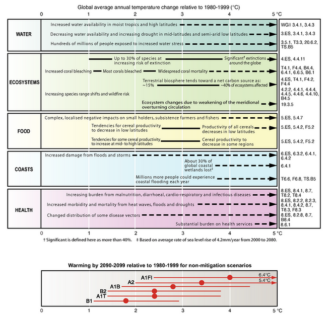
We struggled to make sense of the humanitarian impact of things like “hundreds of millions of people exposed to increased water stress” and “changed distribution of some disease vectors.” Accordingly, we decided to pick the five impacts described in the summaries that qualitatively seemed most worrisome to us to explore and summarize in somewhat greater depth, along with economic assessments that attempt to account holistically for other impacts.
We chose:
- Crop productivity and hunger in Africa
- Floods due to rising sea levels
- Increasing frequency of extreme weather (e.g. hurricanes, heatwaves)
- Adverse effects on health status (e.g. through spreading malaria)
- Significant loss of biodiversity
We chose these five outcomes because they appeared, on the basis of the synthesis report, to be either particularly measurable or to have especially obvious or strong humanitarian impacts.
In our analysis below, we try to report results as far out into the future as they are projected by the Fourth Assessment Report. In most cases, projections go as far out as 2100, but for some outcomes, they only go as far as 2080 or so.
We received feedback (DOCX) on a draft version of this report (PDF) from two expert reviewers who prefer to remain anonymous. Among other issues, they suggested that we investigate increased water stress and incorporate it into our report, which we have done for this version; we have also taken into account their line-by-line feedback. They also pointed out that the sea level rise projections from the AR4 are now considered outdated, and encouraged us to update our write-up to take into account the more recent evidence, which we have down below.
2. Growth scenarios
As discussed below, the projected impacts of climate change depend a lot on how else the world changes over the coming decades. Accordingly, the IPCC Fourth Assessment Report considers six primary “socio-economic development scenarios,” with different projections for population growth, economic growth, and factors related to CO2 emissions (e.g., degree of transition to clean energy):1
- A1 is the scenario most optimistic about per-capita growth; it projects fast economic growth, slow population growth (7.1 billion people in 2100), and quick catch-up in the developing world. Within this broad scenario, three different possibilities for CO2 emissions are considered:
- A1T: Fast transition to clean energy, lower emissions, leading to a 2.4ºC (“likely” range 1.4 – 3.8 ºC) average temperature increase by 2100.
- A1FI: Fossil-fuel intensive economy, high emissions, leading to a 4.0ºC (“likely” range 2.4 – 6.4 ºC) average temperature increase by 2100.
- A1B: medium emissions, between the above two scenarios, leading to a 2.8ºC (“likely” range 1.7 – 4.4 ºC) average temperature increase by 2100.
- A2 is the most pessimistic scenario: slow economic growth, fast population growth (15 billion people in 2100), and slow catch-up in the developing world, with the highest CO2 emissions of any scenario except A1FI above, leading to a 3.4ºC (“likely” range 2.0 – 5.4 ºC) average temperature increase by 2100.
- B1 projects medium-fast economic growth, slow population growth (7.1 billion people in 2100), and quick catch-up in the developing world, with the lowest emissions of any scenario, leading to a 1.8ºC (“likely” range 1.1 – 2.9 ºC) average temperature increase by 2100.
- B2 involves medium-slow economic growth, though higher than in A2 above; medium population growth (10.4 billion people in 2100), and slow catch-up in the developing world. Emissions are at roughly the same level as A1T, which is lower than in any other scenario except B1, leading to a 2.4ºC (“likely” range 1.4 – 3.8 ºC) average temperature increase by 2100.
Broadly speaking, A1 and B1 have faster economic growth and slower population growth than A2 and B2, respectively, while B1 and B2 have lower emissions compared to A1 and A2, respectively.
The following table gives the projected per-capita income levels for different parts of the world. In the slowest-growth scenario, A2, global GDP per capita in 2100 is approximately 4 times as high as global GDP per capita in 1990, and the developing world has roughly 10x as much (though still only half as much as the OECD—a group of rich countries–had in 1990). Under more optimistic growth scenarios—A1 or B1—the developing world ends up with a GDP per capita in 2100 that is 40-60 times higher than in 1990, and 2-3x higher than the OECD had in 1990.
Per-capita income levels in thousands of 1990 US dollars2
| 1990 | |||||||||
|---|---|---|---|---|---|---|---|---|---|
| [ACTUAL] | A1 | A2 | B1 | B2 | A1 | A2 | B1 | B2 | |
| OECD as of 1990 (wealthy countries) | 17.8-20.6 | 50.1 | 34.6 | 49.8 | 39.2 | 109.2 | 58.5 | 79.7 | 61 |
| Developing world | 0.7-1.1 | 15.9 | 3.9 | 10.9 | 8.1 | 66.5 | 11 | 40.2 | 18 |
| World | 3.7-4.0 | 20.8 | 7.2 | 15.6 | 11.7 | 74.9 | 16.1 | 46.6 | 22.6 |
The IPCC Special Report on Emissions Scenarios presents much more detailed information about each of these scenarios.
3. Specific outcomes of climate change
3.1 Crop productivity and hunger in Africa
The IPCC estimates that global warming will have large negative effects on crop productivity in Africa, across a range of socio-economic growth scenarios. However, more of the variation in projected levels of hunger in Africa is driven by socio-economic growth scenarios than by climate change estimates. Across the scenarios considered, the proportion of people at risk of hunger declines by 2080 relative to 2000 even with unmitigated climate change.
By 2100, the IPCC Second Working Group chapter on Africa reports, “parts of the Sahara are likely to emerge as the most vulnerable, showing likely agricultural losses of between 2 and 7% of GDP. Western and central Africa are also vulnerable, with impacts ranging from 2 to 4%. Northern and southern Africa, however, are expected to have losses of 0.4 to 1.3%” (WGII 9.4.4).
Additionally, the chapter reports that (WGII 9.4.4):
- “the area of arid and semi-arid land in Africa could increase by 5-8% (60-90 million hectares).”
- “wheat production is likely to disappear from Africa by the 2080s”
- “In other countries, additional risks that could be exacerbated by climate change include greater erosion, deficiencies in yields from rain-fed agriculture of up to 50% during the 2000-2020 period, and reductions in crop growth period”
- in South Africa, “crop net revenues will be likely to fall by as much as 90% by 2100, with small-scale farmers being the most severely affected. However, there is the possibility that adaptation could reduce these negative effects (Benhin, 2006).”
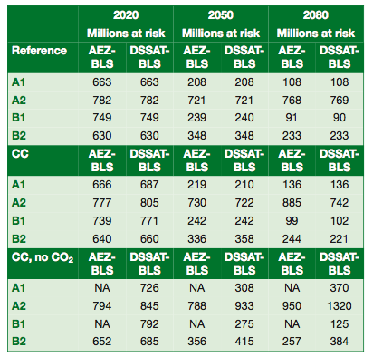
However, the picture presented by the chapter on food is considerably more optimistic. Based on models of the climate, economy, and food system, the IPCC reports the following projections regarding the “number of people at risk of hunger,” with and without climate change:
Millions of people at risk of hunger3
| 2000 | |||||||
|---|---|---|---|---|---|---|---|
| [ACTUAL] | BASELINE PROJECTION | WITH CLIMATE CHANGE | BASELINE PROJECTION | WITH CLIMATE CHANGE | BASELINE PROJECTION | WITH CLIMATE CHANGE | |
| A1 | 824 | 663 | 666-687 | 208 | 210-219 | 108 | 136 |
| A2 | 824 | 782 | 777-805 | 721 | 722-730 | 768-769 | 742-885 |
| B1 | 824 | 749 | 739-771 | 239-240 | 242 | 90-91 | 99-102 |
| B2 | 824 | 630 | 640-660 | 348 | 336-358 | 233 | 221-244 |
Note that this table gives absolute numbers of people at risk of hunger. Across all scenarios, the impact of climate change on hunger is negative (i.e. climate change leads to more hunger). However, expected socio-economic growth plays a large role in the level of vulnerability: in three of the four scenarios considered, hunger declines substantially by 2080 relative to 2000, both with and without the effects of climate change; in A2, which features slow economic growth and fast population growth, the number of people at risk of hunger in 2080, taking into account the effects of climate change, is essentially the same as in 2000. Across all scenarios, hunger is expected to decline as a proportion of the population.4
The effects of climate change in the table are somewhat smaller than might be expected because the models expect the higher atmospheric concentration of CO2 to improve crop growth.5
These impacts are as not as large as the expected gains due to secular growth, so overall hunger is predicted to be less common in 2080 than it is today. However, unmitigated climate change is predicted to lead to substantially greater levels of hunger in 2080 than would occur otherwise.
3.2 Increased water stress
The Fourth Assessment Report synthesis report states that climate change is projected to expose hundreds of millions of people to “increased water stress,”6 though the more detailed Second Working Group chapter reports ambiguity as to the sign of the effect of climate change on the total number of people suffering from water stress,7 with variability across socio-economic assumptions playing a crucial role.
There is less ambiguity about the net humanitarian effects: the Second Working Group chapter on the supply of freshwater reports that “[w]ith respect to water supply, it is very likely that the costs of climate change will outweigh the benefits,”8 and that the impacts of precipitation extremes are expected to occur disproportionately in low-income countries with limited adaptive capacity.9
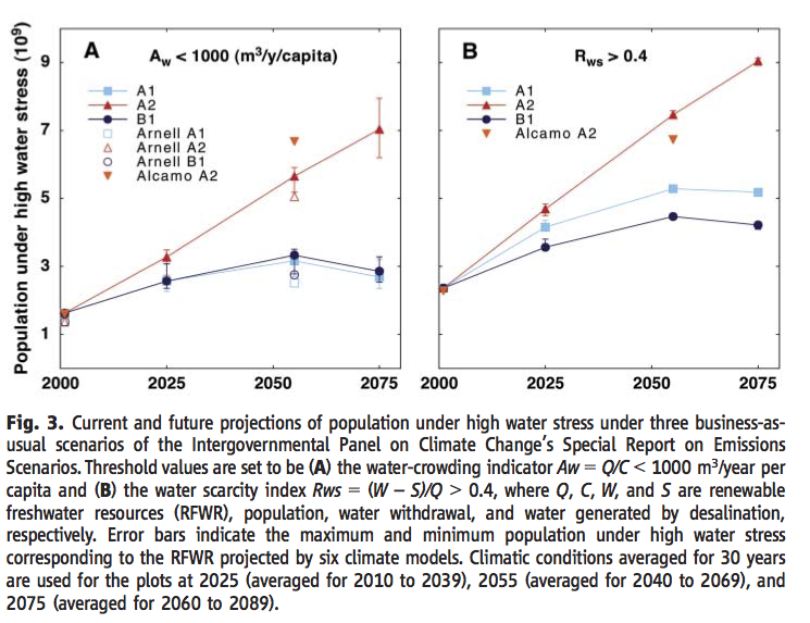
The IPCC cites three sources for figures on the number of people at risk of water stress under various climate scenarios and that extend past 2025 (Vörösmarty et al., 2000 only projects out to 2025), though of the three only Arnell 2004 explicitly compares scenarios with and without climate change to attempt to identify its impact:10
Millions of people living in water-stressed river basins under different socio-economic scenarios over time11
| ~200012 | 202513 | 2050/205514 | 2075/208515 | |||||||||||
|---|---|---|---|---|---|---|---|---|---|---|---|---|---|---|
| BASELINE | A1 | A2 | B1 | B2 | A1 | A2 | B1 | B2 | A1 | A2 | B1 | B2 | ||
| Arnell 200416 | No CC | 1368 17 | 2883 | 3320 | 2883 | 2883 | 3401 | 5596 | 3401 | 3988 | 2860 | 8066 | 2860 | 4530 |
| With CC | 2938 | 2564-3478 | 2368 | 2312-2994 | 2512 | 4351-5747 | 2755 | 2766-3958 | 1667 | 5971-8066 | 2225 | 3234-4634 | ||
| Alcamo 200718 | With CC | 160119 | – | 3576-4286 | – | 3208-3727 | – | 6432-6920 | 4909-5166 | – | 7842-8096 | – | 4617-5962 | |
| Oki and Kanae 200620 | With CC | 1600 | 2500 | 3200 | 2600 | – | 3100 | 5600 | 3400 | – | ||||
This table shows that while scenario A2 consistently has the worst humanitarian outcomes across the sources examined from 2050 on, that is a result of the characteristics of the scenario, rather than the climate change it causes: Arnell’s estimate of A2 water stress outcomes without climate change is similar to or worse than the reported outcomes with climate change (i.e. climate change is predicted to reduce global water stress, though the IPCC notes that costs are still expected to outweigh benefits).21
Important aspects of the impact of climate change on water stress may be inadequately incorporated into these models. For instance, the IPCC reports that irrigation accounts for the majority of global water withdrawals but that there are no global-scale studies of the impact of climate change on irrigation water use.22 Additionally, rural populations in developing countries are expected to be particularly vulnerable to water stress,23 and the projections do not appear to distinguish between populations on the basis of adaptive capacity. Finally, the chapter notes that such figures do not take into account the seasonality of the increasing flows, which are expected to occur during high flow season, and therefore may not be of much benefit during dry seasons.24
On the basis of these studies, the Second Working Group concludes that assumptions about population size and the level of economic growth drive more of the variation in water stress over most of the regions and time periods considered than climate change does:25
Climate change is only one factor that influences future water stress, while demographic, socio-economic, and technological changes may play a more important role in most time horizons and regions. In the 2050s, differences in the population projections of the four SRES scenarios would have a greater impact on the number of people living in water-stressed river basins (defined as basins with per capita water resources of less than 1,000 m3/year) than the differences in the emissions scenarios (Arnell, 2004b)….If water stress is not only assessed as a function of population and climate change, but also of changing water use, the importance of non-climatic drivers (income, water-use efficiency, water productivity, industrial production) increases (Alcamo et al., 2007). Income growth has a much larger impact than population growth on increasing water use and water stress (expressed as the water withdrawal-to-water resources ratio)….
Despite the projections described, we do not feel that we have a strong understanding of the humanitarian impact of water stress as experienced by the 1.4-2.1 billion people currently living in severely stressed basins,26 or what kind of burden adaptation might pose to people placed under water stress in the future. One point of context for the humanitarian weight of water stress is that, as of 1995, 13% of the population of the U.S., 29% of the population of Western Europe, and 24% of the world’s population were classified as living in basins with water stress (under the same definition used in the table above).27
Across scenarios, the number of people experiencing water stress is projected to increase in the future, more as a result of income and population growth than climate change. Climate change is projected to lead to net global reductions in water stress as measured by per capita water availability, though the Second Working Group report predicts that the costs of climate changes on water stress will outweigh the benefits.
3.3 Floods due to rising sea levels
Note: the figures we rely on in the first part of this discussion, from the AR4, are believed to be out of date. See our discussion below.
The Second Working Group chapter on coastal and low-lying areas reports that climate change is likely to lead to a rise in sea levels and an increased risk of flooding in many areas. Assuming that the only form of increased flood protection over time comes from increases in GDP per capita, millions of additional people are expected to be at risk of flooding due to climate change by 2080. We summarize the results, focusing on Asia and Africa because the IPCC projects 0-1 million people at risk of flooding in each of the other regions by 2020.
Average annual number of coastal flood victims in millions (and sea level rise in meters)28
| 1990 | 2020 | 2050 | 2080 | |||||||||||
|---|---|---|---|---|---|---|---|---|---|---|---|---|---|---|
| [Actual] | A1FI (0.05) | A2 (0.05) | B1 (0.05) | B2 (0.06) | A1FI (0.16) | A2 (0.14) | B1 (0.13) | B2 (0.14) | A1FI (0.34) | A2 (0.28) | B1 (0.22) | B2 (0.25) | ||
| Asia | No CC | 9 | 9-12 | 14-20 | 12-17 | 9-13 | 0 | 15-24 | 2 | 1-2 | 0 | 11-18 | 0 | 0-1 |
| With CC | 9-12 | 14-20 | 12-17 | 9-13 | 0 | 16-26 | 2 | 1-2 | 1 | 15-25 | 0 | 0-2 | ||
| Africa | No CC | 1 | 1 | 2-4 | 1 | 3-4 | 0 | 1-2 | 0 | 1-2 | 0 | 0-1 | 0 | 0 |
| With CC | 1 | 2-4 | 1 | 3-4 | 0 | 2-3 | 0 | 1-3 | 2-5 | 4-8 | 1 | 2-4 | ||
| Global Total | No CC | 10 | 10-14 | 17-24 | 13-18 | 12-17 | 0-1 | 16-26 | 2 | 3-4 | 0 | 11-19 | 0 | 1 |
| With CC | 10 | 10-14 | 17-24 | 13-18 | 12-17 | 0 | 18-29 | 2 | 3-5 | |||||
Across all scenarios, climate change is expected to lead to more flooding. In all scenarios except A2, the expected absolute number of people flooded per year in the 2080s, including the effects of sea level rise due to climate change, is less than in 1990 (because of increases in protective capacity due to economic growth). In A2, by contrast, population growth leads to increases in flood victims that are exacerbated by climate change, resulting in a doubling or tripling of total annual number of flood victims by the 2080s, relative to 1990. Under A2, the proportion of people flooded each year remains approximately steady globally after climate change is accounted for, as global population roughly triples (from 5.3 billion in 1990 to 14.2 billion in the 2080s).29
Although the number of people suffering from flooding in A2 is higher than in A1FI, this difference is driven by socio-economic divergence rather than climate change. In 2080, sea level rise under scenario A1FI (34cm) is actually expected to be higher than under A2 (28cm), even though the humanitarian effects are much worse under A2 (essentially because there is a much larger population of very poor people in A2).30 For Africa specifically, climate change is more of a dominant factor.
Note that the risks discussed here concern increased flooding risk; they do not involve significant portions of land becoming completely unusable due to being underwater. The IPCC report does not appear to raise the latter as a major issue; the mention we have seen of this risk in the IPCC report implies that it is primarily a risk over a longer (millennial) time horizon.31 (This is not to say that there’s no chance that such changes could occur in the next century, but rather that the IPCC appears to focus on the risk over a much longer time horizon.)
3.3.1 Updates since the AR4
Our understanding is that the AR4 is now considered outdated with respect to sea level rise,32 and that the Fifth Assessment Report, to be completed in 2014, will feature significantly higher expected sea level rise figures.33
While it’s not clear how substantial an update this is, it does clearly invalidate the claims from the AR4 based on the Nicholls 2004 paper (i.e. the comparison of flooding risk across scenarios and years reported in the table above), which assumed lower sea level rise effects.34 Accordingly, we sought out more recent research on this topic that takes into account the higher expected sea level rise.
Nicholls et al. 2011 take up the issue of updating the assessment of the humanitarian impact of flooding through 2100 based on more recent sea level rise projections, covering estimates between 0.5 and 2 meters (the latter of which is considered an unlikely upper bound).35 Under a pessimistic scenario in which no adaptation is attempted or whatever adaptation attempted fails, climate-change induced sea level rise leads to the displacement of 72 million people (0.9% of the global population) in the 0.5 meter rise scenario and 187 million people (2.4% of the global population) in the 2 meter rise scenario.36 In a more optimistic scenario which, like the Nicholls 2004 estimates quoted in the AR4, assumes that flood protection scales in response to economic growth and rising sea levels, the number of people displaced falls to 41,000 for 0.5 meters of sea level rise and 305,000 for 2 meters of sea level rise.37 However, the assumed adaptation carries large financial costs: 25 billion 1995 USD per year in 2100 for 0.5 meters of sea level rise and 270 billion 1995 USD per year in 2100 for 2 meters of sea level rise,38 which are about 0.005% and 0.05% of the projected global GDP in 2100, respectively.39 Nicholls et al. 2011 does not provide baseline numbers for displacement due to flooding, so we do not have a sense of what kind of proportional increase in displacement 41,000-305,000 additional displaced people represents.
We did not conduct an exhaustive search for literature in this area produced since the release of the AR4, instead focusing on further research on the issue by Nicholls. We anticipate updating our take on this evidence once the full IPCC AR5 is published.
Unmitigated climate change is expected to lead to more people suffering from flooding, but the level of adaptation, which is driven by socio-economic growth scenarios, drives most of the variation in estimates of the number of people subject to flooding in the future. The evidence we have seen does not present a clear picture of whether adaptation or the impact of climate-change-induced sea level rise is likely to have a bigger impact, and accordingly it is unclear whether we should expect net increases or net decreases in the humanitarian impact of flooding over the coming century.
3.4 Increasing frequency of extreme weather (e.g. hurricanes, heat waves)
Although extreme weather is discussed in the IPCC’s Fourth Assessment Report, the IPCC issued a more recent document, “Managing the Risks of Extreme Events and Disasters to Advance Climate Change Adaptation (SREX),” focused specifically on extreme events, so we referred to that document for information about this outcome.
The IPCC states that it is difficult to attribute any increases in extreme weather to climate change, because extreme climate events are rare,40 but that it is virtually certain that – in most regions – extremely hot days and heat waves will become more frequent while extremely cold days become less frequent.41
The change in frequency of extremely hot days depends on the socio-economic scenario modeled (which drives the level of emissions), but under high-emissions scenarios, a day so hot that it would only happen once in every twenty years in 1990 would occur every 2 years in 2100, and the once-in-twenty-years temperatures are expected to rise by about 2 to 5°C.42
Other projected impacts include:
- Precipitation: “For a range of emission scenarios (A2, A1B, and B1), projections indicate that it is likely that a 1-in-20 year annual maximum 24-hour precipitation rate will become a 1-in-5 to -15 year event by the end of 21st century in many regions. Nevertheless, increases or statistically non-significant changes in return periods are projected in some regions.” (SREX 149)
- Tropical cyclones: Information about tropical cyclones is relatively sparse in the historical record, but SREX reports that it is likely that the intensity of cyclones (in terms of rainfall and maximum wind speed) will increase while the number of cyclones will remain constant or decline (SREX 163).
- Droughts: SREX expresses medium confidence that there have been changes in some regions of the world since 1950 in the pattern of droughts (some positive, some negative), low confidence that climate change has already caused changes in drought patterns in individual regions, and medium confidence that climate change will lead to an increase in duration and intensity of droughts in some regions (including central North America and southern Africa) (pgs 174-175).
Economic and humanitarian losses due to extreme weather events are not well-quantified, but SREX reports high confidence that “[i]ncreasing exposure of people and economic assets has been the major cause of long-term increases in economic losses from weather- and climate-related disasters” (pg 269). (Here “increasing exposure” refers to change in geographic distribution of assets rather than due to weather becoming worse.) In the cases for which SREX presents the most thorough information (primarily in the developed world), it appears that changes in exposure (presumably due to differing patterns of socio-economic development) are generally expected to drive larger changes in economic losses through 2040 than climate change does (SREX 272):

This a short time horizon, however, and the types of disasters covered are not the ones that have historically been associated with the largest humanitarian impacts, which have been in the developing world.
Historically, natural disasters have had disproportionate effects on low-income countries, causing higher fatality rates and destroying a greater portion of GDP (pg 265). Between 1970 and 2008, greater than 95% of disaster deaths were in developing countries (pg 265). Between 1980 and 2004, the global economic losses dues to weather and climate disasters (which tend to be mostly in the developed world) have grown faster than the population or the economy, while at the same time the number of lives lost (mostly in the developing world) has declined (pg 269).
It is not clear why the number of lives lost due to extreme weather events has declined. Possible explanations may include “gradual improvements in warnings and emergency management, building regulations, and changing lifestyles (such as the use of air conditioning), and the almost instant media coverage of any major weather extreme that may help reduce losses” (pg 269). We would generally expect these trends to continue due to ongoing economic growth, potentially mitigating some future impacts of climate change due to extreme weather.
Accordingly, we see the research on extreme weather events as fitting the same general pattern as flooding: climate change is projected to have substantial negative impacts (especially leading to higher temperature extremes), but difficult-to-assess growth projections dominate our assessment of future vulnerability.
3.5 Adverse effects on health status (e.g., through spreading malaria)
The two best-understood kinds of health effects of climate change appear to be heat and cold deaths and infectious disease (e.g. on malaria or dengue fever). The expected health effects of climate change are expected to be large, negative, and fall disproportionately on low-income countries (WGII 8.ES), while the effects of socio-economic changes are expected to dominate the effects of climate change in the future (WGII 8.3.2).
3.5.1 Heat and cold deaths
Climate change is expected to increase the number of heat-related deaths, especially amongst the elderly, and reduce the number of cold-related deaths (WGII 8.4.1.3), though quantified estimates are not provided on a global basis – instead, studies of particular areas are cited. For example, in the UK, heat deaths are predicted to rise by ~3000 per year by 2080, while cold deaths are predicted to fall by ~30,000 per year; heat-related deaths in Los Angeles are expected to rise from ~165/year in the 1990s to 319-1182 per year in the 2080s. Note that a heat wave in Europe in 2003 is believed to have caused roughly 35,000 deaths, mostly amongst those over the age of 75 (WGII 8.2.1.1). Heat-related deaths are expected to increase partly because of demographics, due to the higher risk that the elderly face.43
3.5.2 Malaria
Regarding malaria, the IPCC says, “trends in population dominate calculations of the possible consequences of climate change” (WGII 8.3.2). van Lieshout et al. 2004, the source cited by the IPCC for global malaria projections, does not separate out the impacts of population growth from climate change. It predicts that, by the 2080s, climate change will lead to (van Lieshout et al. 2004 Table 2):
- regions that are at risk of malaria in at least one month a year expanding across all scenarios, to cover between 227 million (scenario A1FI, fast fossil-fuel-intensive economic growth) and 416 million (scenario A2, slow economic growth and fast population growth) additional people.
- varying effects on the size of regions that are at risk of malaria in at least three months a year:
- 100 million additional people (A1FI)
- 141 million fewer people (A2)
- 153 million fewer people (B1, medium-fast economic growth, slow population growth, and low emissions)
- 31 million additional people (B2, medium economic and population growth and medium-low emissions).
Although van Lieshout et al. 2004 does not explicitly compare the effects of population growth and climate change on population at risk of malaria, we can infer that population growth has a bigger impact than climate change. The 2080 population of South Asia alone differs by more than 800 million between scenarios A1 and A2 (Fig 3), and the entire region is at risk of malaria for at least one month per year regardless of the impacts of climate change (Fig 6 and Table 2), implying that population growth is a significantly larger factor in driving malaria vulnerability than climate change is. Also, the authors do not model any changes in capacity over time, so any progress on malaria control that may occur with or without climate change is not included in the projection.
3.5.3 Dengue fever
Regarding dengue fever, there is some confusion due to an apparent misreading of a study (on the part of the IPCC),44 but it appears to us that the authors predict that the total number of people living in regions at risk of dengue fever will go from ~1.5 billion (1990 baseline) to 5-6 billion (2085), with 2 billion of that coming from population growth alone and the remaining 1.5-2.5 billion coming from climate change.45 The authors modeled only one growth scenario, and as with malaria, did not attempt to model the effects of adaptive capacity (e.g., control efforts).
3.5.4 Adaptive capability
A major question regarding all three of the above impacts is that of adaptive capability: improved control efforts, safety measures and care options due to increased wealth. For example, over the last century, the areas at risk of malaria have declined substantially (malaria has been eliminated in the U.S. and Europe, among other places):

We expect that unmitigated climate change would have large negative impacts on health, particularly in low-income countries, during the coming century, but as with flooding and extreme events, difficult-to-assess growth projections dominate our assessment of future vulnerability.
3.6 Significant loss of species and biodiversity
The IPCC predicts that climate change will lead to a substantial number of species extinctions (e.g. potentially in the region of 20-30% of all species) and substantial loss of biodiversity by 2100 (WGII 4.ES).
The impact of this biodiversity loss on humans is a key uncertainty in our take on the humanitarian impact of climate change. Because species extinction is irreversible, it represents one way in which people living in 2100 could be undeniably worse off than people living today: they may have a smaller pool of animal and plant life on which to draw for research, cultural and economic activity. We are not aware of any estimate of the humanitarian value of the particular species that are at risk. (The Stern Review, discussed below, may include biodiversity as part of its assessment of the “non-market” impacts of climate change, but the biodiversity costs are not disaggregated.46) The Fourth Assessment Report does point to an estimate of the total value of ecosystem goods and services as approximately equal to the global gross national product, but does not provide an estimate of the value of biodiversity expected to be lost due to climate change (WGII 4.5).
Note that these estimates of species losses are primarily made using “climate envelope models,” which use climate change models and information about the geographic distribution of species to estimate when the conditions in which they currently reside are likely to cease to exist (i.e. when the “climate envelope” in which they live will be eliminated) (WGII 4.4.11). Many of the expected species losses in these models come from endemic species—ones that are restricted to narrow geographic and climatic areas—which can be especially sensitive to climatic changes.
Because these species represent a disproportionately small fraction of the planet’s biomass and they have generally not been cultivated at a large scale, we expect that the average humanitarian value of the species at risk is likely to be less than the average humanitarian value of all species, though the value of their biodiversity alone may nonetheless be enormous.
Over the next century, biodiversity loss is expected to be driven more by climate change than other socio-economic drivers (e.g. deforestation or land-use changes), and the net effects of climate change and socio-economic growth on biodiversity are expected to be large and negative (WGII 4.4.11).
4. Economic welfare
In addition to examining the IPCC’s projections regarding specific impacts, we also examined its discussion of the overall effect on the world economy. Climate change has large predicted negative effects across all scenarios, but the socio-economic growth scenarios themselves have a much larger influence on future welfare than climate change does. Unmitigated climate change appears unlikely (according to IPCC projections) to eliminate the large secular gains projected by all the IPCC socio-economic scenarios over the 21st century.
The chapter of the Fourth Assessment Report that analyzes economic impacts focuses particularly on the estimates from the Stern Review, a 2007 report compiled for the UK government (WGII 20.6.1):
A 20% decrease in per capita consumption would be nearly equivalent to the decline experienced by the U.S. during the Great Depression, without the associated recovery.
Although the IPCC does not quote the Stern Review to this effect, the quoted impacts of climate change are taking into account projections out past 2200, a century further into the future than the other projections the Fourth Assessment Report makes. Using a model that takes into account the risk of catastrophe and non-market impacts and worse-than-expected climate change (i.e. everything except equity weights from the quote above), the Stern review projects a 2.9% reduction in per capita GDP in 2100.47 Using the Stern Review’s back-of-the-envelope equity weights, that would imply an equivalent loss of welfare in 2100 of about 4%.48
What does a 4% loss of GDP per capita really mean? The Stern Review is based on a probabilistic simulation, but it takes a particular socio-economic growth model, SRES scenario A2, which features fast population growth and slow economic growth, as its base (Stern Review pg 154). Of the six major scenarios included in the IPCC Fourth Assessment Report, A2 has the second worst climate change impacts (after only A1FI, the most fossil fuel-intensive fast-growth scenario). A2 also features the worst humanitarian outcomes of the SRES scenarios, with slower convergence of the developing world and slower overall economic growth. Prior to taking into account climate change, the GDP per capita of the developing world in 2100 under scenario A2 is $11,000; a 4% hit from climate change drops it to $10,560. In 1990, GDP per capita in the developing world was about $1,000.
All told, on a 2100 time-scale, the variation across socio-economic scenarios dwarfs climate change in terms of their impact on economic outcomes. The four families of scenarios differ by 6 times in the expected level of GDP per capita in 2100. By way of contrast, the impact of climate change in family A2 (the second worst of the six considered by the IPCC) is about 4% of GDP per capita in 2100: this is about 100 times smaller than the variation across the socio-economic scenarios. Even with projected negative impacts of climate change in the range of 4%, the developing world is roughly 10 times wealthier in 2100 than in 1990 in scenario A2, which is the worst scenario in terms of humanitarian growth. In more optimistic growth scenarios, such as A1 or B1, the developing world is 40-60 times richer in 2100 than in 1990 (and 2-3 times richer than the OECD was in 1990).49
We would guess that this dominance would also hold on a longer time-scale (e.g. out to 2200, as the Stern Review goes), because both economic growth and the impacts of climate change are compounding, but the SRES projections do not go out that far.
5. Conclusion
Across all of the outcomes we looked at, the effects of unmitigated climate change are projected to be very large and negative—enough to provide strong support for policy action to mitigate climate change.
Assumptions about socio-economic growth and adaptation play an important role in predicting future vulnerability. In the case of two of the outcomes that we examined (hunger and overall assessments of economic losses), growth scenarios drive the overall outcomes, resulting in projected net improvements relative to 2000 when large losses due to unmitigated climate change and large gains due to economic growth are both taken into account. In three other cases (flooding, extreme weather, and health effects), the evidence is less clear: the size of the expected negative impacts of climate change depend substantially on the level of adaptation and growth that is expected, but the net expected effects are ambiguous. In the case of biodiversity, not only are the projected effects of climate change unambiguously negative, but the IPCC expects limited compensation from socio-economic growth, resulting in a large net loss by 2100. Like biodiversity, water stress is expected to be more of a problem in the future than it is today, though the role of climate change is less significant than projected increases in population and income.
6. Sources
Alcamo, Joseph, Martina Flörke, and Michael Märker. 2007. Future long-term changes in global water resources driven by socio-economic and climatic changes. Hydrological Sciences Journal 52(2): 247-275.
Arnell, Nigel W. 2004. Climate change and global water resources: SRES emissions and socio-economic scenarios. Global Environmental Change 14: 31-52.
Berger, Eric. 2012. Draft IPCC report leaked, shows substantial warming. – Source
Hales, Simon, et al. 2002. Potential effect of population and climate changes on global distribution of dengue fever: an empirical model. Lancet 360(9336): 830-834.
IPCC, 2007. Climate Change 2007: Impacts, Adaptation and Vulnerability. Contribution of Working Group II to the Fourth Assessment Report of the Intergovernmental Panel on Climate Change. M.L. Parry, O.F. Canziani, J.P. Palutikof, P.J. van der Linden and C.E. Hanson, Eds., Cambridge University Press, Cambridge, UK.
IPCC, 2007. – Source [Core Writing Team, Pachauri, R.K and Reisinger, A. (eds.)]. IPCC, Geneva, Switzerland.
IPCC, 2012. – Managing the Risks of Extreme Events and Disasters to Advance Climate Change Adaptation. A Special Report of Working Groups I and II of the Intergovernmental Panel on Climate Change [Field, C.B., V. Barros, T.F. Stocker, D. Qin, D.J. Dokken, K.L. Ebi, M.D. Mastrandrea, K.J. Mach, G.-K. Plattner, S.K. Allen, M. Tignor, and P.M. Midgley (eds.)]. Cambridge University Press, Cambridge, UK.
Nicholls, Robert J. 2004. Coastal flooding and wetland loss in the 21st century: changes under the SRES climate and socio-economic scenarios. Global Environmental Change 14(1): 69-86.
Nicholls, Robert J., et al. 2011. Sea-level rise and its possible impacts given a ‘beyond 4°C world’ in the twenty-first century. Philosophical Transactions of the Royal Society A 369: 161-181.
Nordhaus, William D. 2007. A Review of the Stern Review on the Economics of Climate Change. Journal of Economic Literature (45): 686-702.
Oki, Taikan, and Shinjiro Kanae. 2006. Global hydrological cycles and world water resources. Science 313: 1068-1072.
Rahmstorf, Stefan, Grant Foster and Anny Cazenave. 2012. Comparing climate projections to observations up to 2011. Environmental Research Letters 7: 044035.
Stern, Nicholas, 2007. Source Cambridge University Press, Cambridge.
van Lieshout, M., et al. 2004. Climate change and malaria: analysis of the SRES climate and socio-economic scenarios. Global Environmental Change 14(1): 87-99.