Semi-Informative Priors Over AI Timelines

One of Open Phil’s major focus areas is technical research and policy work aimed at reducing potential risks from advanced AI. As part of this, we aim to anticipate and influence the development and deployment of advanced AI systems.

To inform this work, I have written a report developing one approach to forecasting when artificial general intelligence (AGI) will be developed. This is the full report. An accompanying blog post starts with a short non-mathematical summary of the report, and then contains a long summary.

1 Introduction

1.1 Executive summary

The goal of this report is to reason about the likely timing of the development of artificial general intelligence (AGI). By AGI, I mean computer program(s) that can perform virtually any cognitive task as well as any human,1 for no more money than it would cost for a human to do it. The field of AI is largely held to have begun in Dartmouth in 1956, and since its inception one of its central aims has been to develop AGI.2

I forecast when AGI might be developed using a simple Bayesian framework, and choose the inputs to this framework using commonsense intuitions and reference classes from historical technological developments. The probabilities in the report represent reasonable degrees of belief, not objective chances.

One rough-and-ready way to frame our question is this:

Suppose you had gone into isolation in 1956 and only received annual updates about the inputs to AI R&D (e.g. # of researcher-years, amount of compute3 used in AI R&D) and the binary fact that we have not yet built AGI? What would be a reasonable pr(AGI by year X) for you to have in 2021?

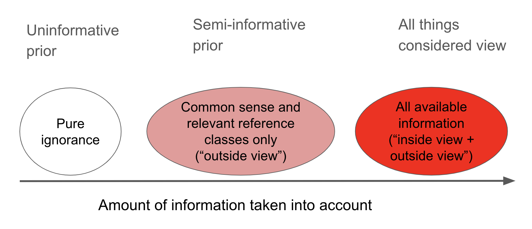
There are many ways one could go about trying to determine pr(AGI by year X). Some are very judgment-driven and involve taking stances on difficult questions like “since AI research began in 1956, what percentage of the way are we to developing AGI?” or “what steps are needed to build AGI?”. As our framing suggests, this report looks at what it would be reasonable to believe before taking evidence bearing on these questions into account. In the terminology of Daniel Kahneman’s Thinking, Fast and Slow, it takes an “outside view” approach to forecasting, taking into account relevant reference classes but not specific plans for how we might proceed.4 The report outputs a prior pr(AGI by year X) that can potentially be updated by additional evidence.5

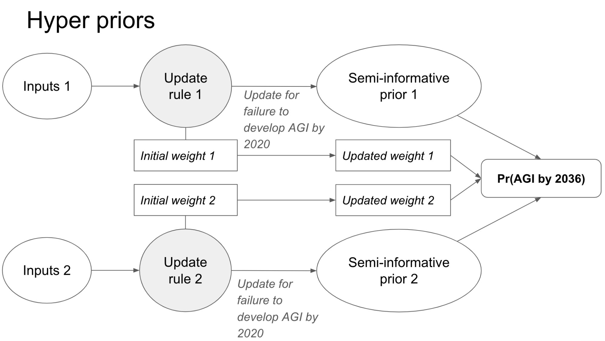
Our framework only conditions on the inputs to AI R&D – in particular the time spent trying to develop AGI, the number of AI researchers, and the amount of compute used – and the fact that we haven’t built AGI as of the end of 2020 despite a sustained effort.6 I place subjective probability distributions (“beta-geometric distributions” ) over the amount of each input required to develop AGI, and choose the parameters of these distributions by appealing to analogous reference classes and common sense. My most sophisticated analysis places a hyperprior over different probability distributions constructed in this way, and updates the weight on each distribution based on the observed failure to develop AGI to date.

For concreteness and historical reasons,7 I focus throughout on what degree of belief we should have that AGI is developed by the end of 2036: pr(AGI by 2036).8 My central estimate is about 8%, but other parameter choices I find plausible yield results anywhere from 1% to 18%. Choosing relevant reference classes and relating them to AGI requires highly subjective judgments, hence the large confidence interval. Different people using this framework would arrive at different results.

To explain my methodology in some more detail, one can think of inputs to AI R&D – time, researcher-years, and compute – as “trials” that might have yielded AGI, and the fact that AGI has not been developed as a series of “failures”.9 Our starting point is Laplace’s rule of succession, sometimes used to estimate the probability that a Bernoulli “trial” of some kind will “succeed” if n trials have taken place so far and f have been “failures”. Laplace’s rule places an uninformative prior over the unknown probability that each trial will succeed, to express a maximal amount of uncertainty about the subject matter. This prior is updated after observing the result of each trial. We can use Laplace’s rule to calculate the probability that AGI will be developed in the next “trial”, and so calculate pr(AGI by 2036).10

I identify severe problems with this calculation. In response, I introduce a family of update rules, of which the application of Laplace’s rule is a special case.11 Each update rule can be updated on the failure to develop AGI by 2020 to give pr(AGI by year X) in later years. When a preferred update rule is picked out using common sense and relevant reference classes, I call the resultant pr(AGI by year X) a ‘semi-informative prior’. I sometimes use judgments about what is a reasonable pr(AGI by year X) to constrain the inputs, trying to achieve reflective equilibrium between the inputs and pr(AGI by year X).

 

 

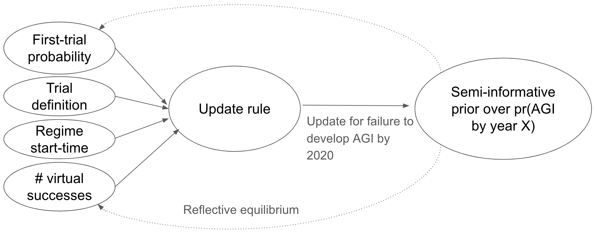
A specific update rule from the family is specified by four inputs: a first-trial probability (ftp), a number of virtual successes, a regime start-time, and a trial definition.

• The first-trial probability gives your odds of success on the first trial. Roughly speaking, it corresponds to how easy you thought AGI would be to develop before updating on the observed failure to date.
  • The main problem with Laplace’s rule is that it uses a first-trial probability of 50%, which is implausibly high and results in inflated estimates of pr(AGI by 2036).
• The number of virtual successes influences how quickly one updates away from the first-trial probability as more evidence comes in (etymology explained in the report).
• The regime start-time determines when we start counting successes and failures, and I think of it in terms of when serious AI R&D efforts first began.
• The trial definition specifies the increase of an R&D input corresponding to a “trial” – e.g. ‘a calendar year of time’ or ‘a doubling of the compute used to develop AI systems’.

I focus primarily on a regime start-time of 1956, but also do sensitivity analysis comparing other plausible options. I argue that a number of virtual successes outside of a small range has intuitively odd consequences, and that answers within this range don’t change my results much. Within this range, my favored number of virtual successes has the following implication: if the first-trial probability is 1/X, then pr(AGI in the first X years) 50%.

The first-trial probability is much harder to constrain, and plausible variations drive more significant differences in the bottom line than any other input. Taking a trial to be a ‘a calendar year of time’, I try to constrain the first-trial probability by considering multiple reference classes for AGI – for example “ambitious but feasible technology that a serious STEM field is explicitly trying to build” and “technological development that has a transformative effect on the nature of work and society” – and thinking about what first-trial probability we’d choose for those classes in general. On this basis, I favor a first-trial probability in the range [1/1000, 1/100], and feel that it would be difficult to justify a first-trial probability below 1/3000 or above 1/50. A first-trial probability of 1/300 combined with a 1956 regime start-time and 1 virtual success yields pr(AGI by 2036) = 4%.

I consider variations on the above analysis with trials defined in terms of researcher-years and compute used to develop AI, rather than time.12 I find that these variations can increase the estimate of pr(AGI by 2036) by a factor of 2 – 4. I also find that the combination of a high first-trial probability and a late regime start-time can lead to much higher estimates of pr(AGI by 2036).

 

TRIAL DEFINITION	LOW FTP	CENTRAL FTP	HIGH FTP	HIGH FTP AND LATE START-TIME: 2000
Calendar year	1%	4%	9%	12%
Researcher-year	2%	8%	15%	25%
Compute13	2%	15%	22%	28%

Here are my central estimates for pr(AGI by year X) out to 2100, which rely on crude empirical forecasts past 2036.14

 

 

To form an all-things-considered judgment, I place a hyperprior over different update rules (each update rule is determined by the four inputs). The hyper-prior assigns an initial weight to each update rule and then updates these weights based on the fact that AGI has not yet been developed.15

The inputs leading to low-end, central, and high-end estimates are summarized in this table (outputs in bold, inputs in standard font).

 

	LOW-END	CENTRAL	HIGH-END
First-trial probability (trial = 1 calendar year)	1/1000	1/300	1/100
Regime start-time	1956	85% on 1956, 15% on 2000	20% on 1956, 80% on 2000
Initial weight on time update rule	50%	30%	10%
Initial weight on researcher-year update rule	30%	30%	40%
Initial weight on compute update rule	0%	30%	40%
Initial weight on AGI being impossible	20%	10%	10%
pr(AGI by 2036)	1%	8%	18%
pr(AGI by 2100)	5%	20%	35%

The four rows of weights are set using intuition, again highlighting the highly subjective nature of many inputs to the framework. I encourage readers to use this tool to see the results of their preferred inputs.

Much of the report investigates and confirms the robustness of these conclusions to a variety of plausible variations on the analysis and anticipated objections. For example, I consider models where developing AGI is seen as a conjunction of independent processes or a sequence of accomplishments; some probability is reserved for AGI being impossible; different empirical assumptions are used to fix the first-trial probability for various trial definitions. I also consider whether using this approach would produce absurd consequences in other contexts (e.g. what does analogous reasoning imply about other technologies?), whether it matters that the framework is discrete (dividing up continuous R&D inputs into arbitrarily sized chunks), and whether it’s a problem that the framework models AI R&D as a series of Bernoulli trials. On this last point, I argue in Appendix 12 that using a different framework would not significantly change the results because my bottom line is driven by my choice of inputs to the framework rather than my choice of distribution.

One final upshot of interest from the report is that the failure to develop AGI to date is not strong evidence for low pr(AGI by 2036). In this framework, pr(AGI by 2036) lower than ~5% would primarily be a function of one’s first-trial probability. In other words, a pr(AGI by 2036) lower than this would have to be driven by an expectation — before AI research began at all — that AGI would probably take hundreds or thousands of years to develop.16

Acknowledgements: My thanks to Nick Beckstead, for prompting this investigation and for guidance and support throughout; to Alan Hajek, Jeremy Strasser, Robin Hanson, and Joe Halpern for reviewing the full report; to Ben Garfinkel, Carl Shulman, Phil Trammel, and Max Daniel for reviewing earlier drafts in depth; to Ajeya Cotra, Joseph Carlsmith, Katja Grace, Holden Karnofsky, Luke Muehlhauser, Zachary Robinson, David Roodman, Bastian Stern, Michael Levine, William MacAskill, Toby Ord, Seren Kell, Luisa Rodriguez, Ollie Base, Sophie Thomson, and Harry Peto for valuable comments and suggestions; and to Eli Nathan for extensive help with citations and the website. Lastly, many thanks to Tom Adamczewski for vetting the calculations in the report and building the interactive tool.

1.2 Structure of report

Section 2 applies Laplace’s rule of succession to calculate pr(AGI by year X). I call the result an ‘uninformative prior over AGI timelines’, because of the rule’s use of an uninformative prior. This approach yields pr(AGI by 2036) of 20%.

Section 3 identifies a family of update rules of which the previous application of Laplace’s rule is a special case, highlighting some arbitrary assumptions made in Section 2. When a preferred update rule from the family is picked out using common sense and relevant reference classes, I call the resultant pr(AGI by year X) a ‘semi-informative prior over AGI timelines’.

 

 

Section 3 also identifies severe problems with the application of Laplace’s rule to AGI timelines, but suggests that these do not arise in context of the broader family of update rules. Lastly, it conducts a sensitivity analysis which highlights that one input is particularly important to pr(AGI by 2036) – the first-trial probability.

Section 4 describes what I think is the correct methodology for constraining the first-trial probability in principle, and discusses a number of considerations that might help the reader constrain their own first-trial probability in practice. I then explain the range of values for this input that I currently favor. Much more empirical work could be done to inform this section; the considerations I discuss are merely suggestive. This is somewhat unfortunate as the first-trial probability is the single most important determinant of your bottom line pr(AGI by 2036) in this framework.

Section 5 analyzes how much the number of virtual successes and regime start-time affect the bottom line, once you’ve decided your first-trial probability. Its key conclusion is that they don’t matter very much.

Section 6 considers definitions of a ‘trial’ researcher-years and compute. (Up until this point a ‘trial’ was defined as a year of calendar time.) More specifically, it defines trials as percentage increases in i) the total number of AI researcher-years, and ii) the compute used to develop the largest AI systems.17 I find that each successive trial definition increases the bottom line, relative to those before it. This is because the relevant quantities are all expected to change rapidly over the next decade, matching recent trends,18 and so an outsized number of ‘trials’ will occur.

Section 7 extends the model in three ways, and evaluates the consequences for the bottom line. First, it explicitly models AGI as conjunctive. In this simple extension, multiple goals must be achieved to develop AGI and each goal has its own semi-informative prior. I also consider models where these goals must be completed sequentially. The main consequence is to dampen the probability of developing AGI in the initial decades of development. These models output similar values for pr(AGI by 2036), as they make no assumption about how many conjuncts are completed as of 2020.

 

 

Second, Section 7 places a hyperprior over multiple semi-informative priors. The hyperprior assigns initial weights to the semi-informative priors and updates these weights based on how surprised each prior is by the failure to develop AGI to date. The semi-informative priors may differ in their first-trial probability, their trial definition, or in other ways. Thirdly, it explicitly models the possibility that AGI will never be developed, which slightly decreases pr(AGI by 2036).

 

 

Section 8 concludes, summing up the main factors that influence the bottom line. My own weighted average over semi-informative priors implies that pr(AGI by 2036) is about 8%. Readers are strongly encouraged to enter their own inputs using this tool.

The appendices cover a number of further topics, including:

• In what circumstances does it make sense to use the semi-informative priors framework (here)?
• Is it a problem that the framework unrealistically assumes that AI R&D is a series of Bernoulli trials (here)?
• Is it a problem that the framework treats inputs to AI R&D as discrete, when in fact they are continuous (here)?
• Does this framework assign too much probability to crazy events happening (here)?
• Is the framework sufficiently sensitive to changing the details of the AI milestone being forecast? I.e. would we make similar predictions for a less/more ambitious goal (here)?
• How might other evidence make you update from your semi-informative prior (here)?

Appendix 12 is particularly important. It justifies the adequacy of the semi-informative priors framework, given this report’s aims, in much greater depth. It argues that, although the framework models the AGI development process as a series of independent trials with an unknown probability success, the framework’s legitimacy and usefulness does not depend upon this assumption being literally true. To reach this conclusion, I consider the unconditional probability distributions over total inputs (total time, total researcher-years, total compute) that the semi-informative priors framework gives rise to. This turns out to correspond to the family of beta-geometric distributions. Each semi-informative prior corresponds to one such beta-geometric distribution, and we can consider these distributions as fundamental (rather than derivative on the assumption that AI R&D is a series of trials). I argue that this class of unconditional probability distributions is sufficiently expressive for the purposes of this report.

Three academics reviewed the report. I link to their reviews in Appendix 15.

Note: throughout the report, potential objections and technical subtleties are often discussed in footnotes to keep the main text more readable.

2 Uninformative priors over AGI timelines

2.1 The sunrise problem

The polymath Laplace introduced the sunrise problem:

Suppose you knew nothing about the universe except whether, on each day, the sun has risen. Suppose there have been N days so far, and the sun has risen on all of them. What is the probability that the sun will rise tomorrow?

Just as we wish to bracket off information about precisely how AGI might be developed, the sunrise problem brackets off information about why the sun rises. And just as we wish to take into account the fact that AGI has not yet been developed as of the start of 2020, the sunrise problem takes into account the fact that the sun has risen on every day so far.

2.1.1 Naive solution to the sunrise problem

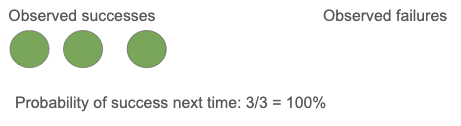
One might think the probability of an event is simply the fraction of observations you’ve made in which it occurs: (number of observed successes) / (number of observations).19

 

 

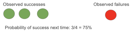
In the sunrise problem, we’ve observed N successes and no failures, so this naive approach would estimate the probability that the sun rises tomorrow as 100%. This answer is clearly unsatisfactory when N is small. For example, observing the sun rise just three times does not warrant certainty that it will rise the next day.

 

2.1.2 Laplace’s solution to the sunrise problem: the rule of succession

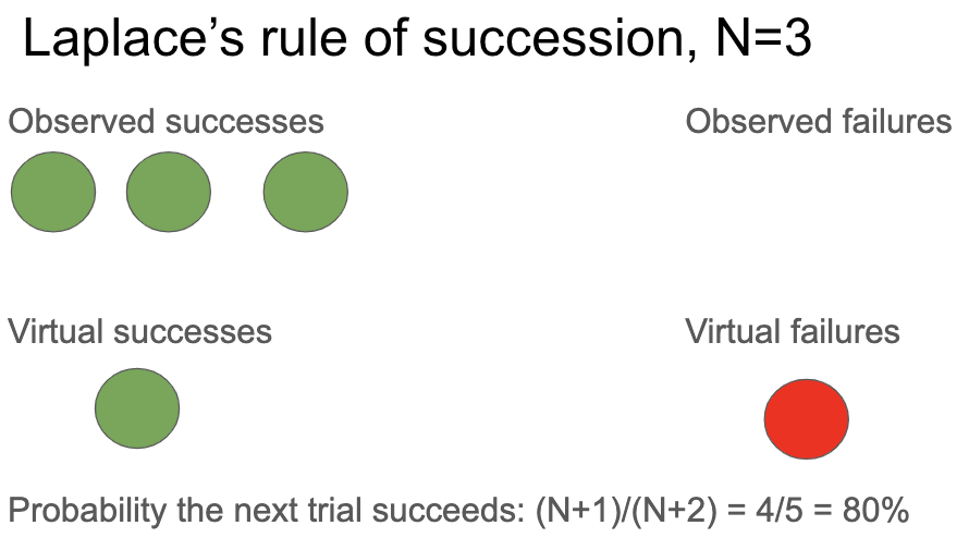
Laplace’s proposed solution was his rule of succession. He assumes that each day there is a ‘trial’ with a constant but unknown probability p that the sun rises. To represent our ignorance about the universe, Laplace recommends that our initial belief about p is a uniform distribution in the range [0, 1]. According to this uninformative prior, p is equally likely to be between 0 and 0.01, 0.5 and 0.51, and 0.9 and 0.91; the expected value of p is E(p) = 0.5.

When you update this prior on N trials where the sun rises and none where it does not,20 your posterior expected value of p is:

\( E(p)=(N+1)/(N+2) \)

In other words, after seeing the sun rise without fail N times in a row, our probability that it will rise on the next day is \( (N + 1) / (N + 2) \).

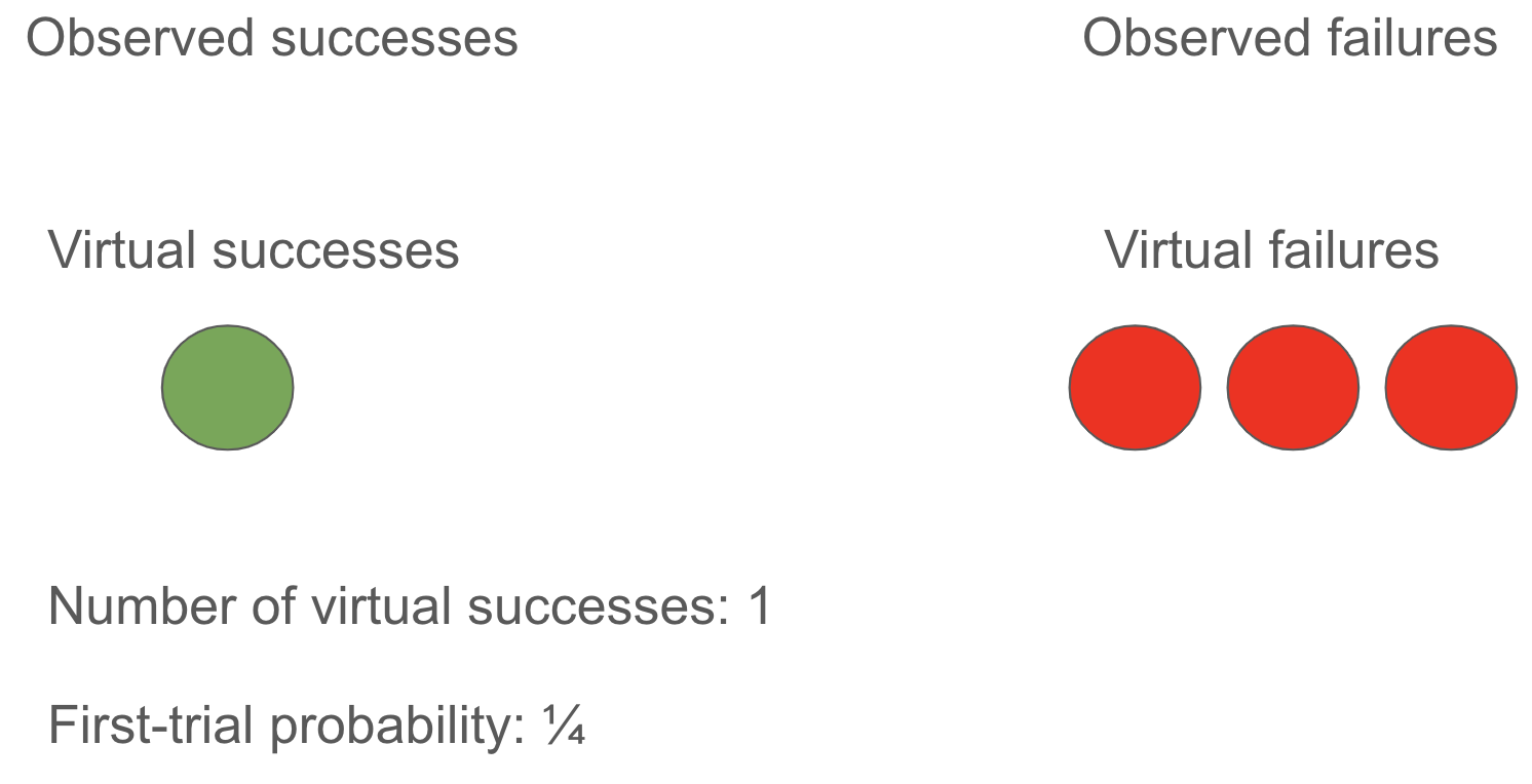
One way to understand this formula is to suppose that, before we saw the sun rise on the first day, we made two additional virtual observations.21 In one of these the sun rose, in another it didn’t. Laplace’s rule then says the probability the sun rises tomorrow is given by the fraction of all past observations (both virtual and actual) in which the sun rose.

 

2.2 Applying Laplace’s rule of succession to AGI timelines

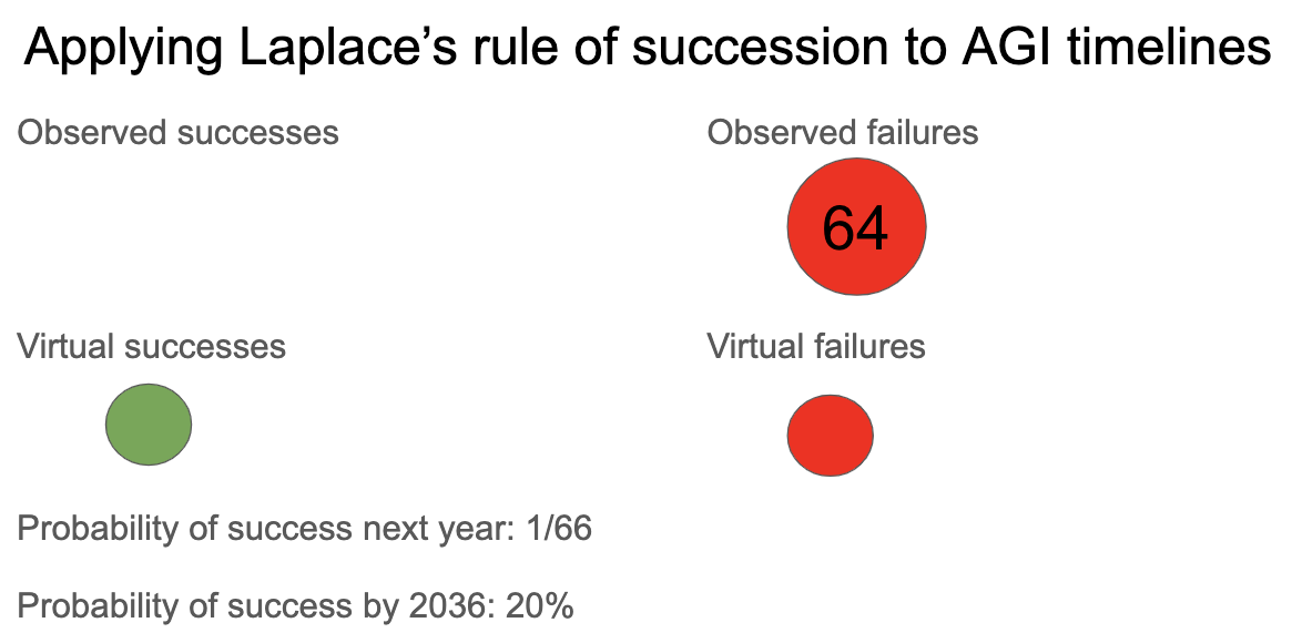
I want to estimate pr(AGI by 2036).22 Rather than observing that the sun has risen for N days, I have observed that AI researchers have not developed AGI with N years of effort. The field of AI research is widely held to have begun in Dartmouth in 1956, so it is natural to take N = 64. (The choice of a year – rather than e.g. 1 month – is arbitrary and made for expositional purposes. The results of this report don’t depend on such arbitrary choices, as discussed in the next section.)

By analogy with the sunrise problem, I assume there’s been some constant but unknown probability p of creating AGI each year. I place a uniform prior probability distribution over p to represent my uncertainty about its true value, and update this distribution for each year that AGI hasn’t happened.23

The rule of succession implies that the chance AGI will again not be developed on the next trial is (N + 1) / (N + 2) = 65/66. The chance it will not be developed in any of the next 16 trials is 65/66 × 66/67 × … × 81/82 = 0.8, and so pr(AGI by 2036) = 0.2.

An equivalent way to think about this calculation is that, after observing 64 failed trials, our belief about chance of success in the next trial E(p) is 1/66. This is the fraction of our actual and virtual observations that are successes. So our probability of developing AGI next year is 1/66. We combine the probabilities for the next 16 years to get the total probability of success.

 

 

The next section discusses some significant problems with this application of Laplace’s rule of succession. These problems will motivate a more general framework, in which this calculation is a special case.

3 Semi-informative priors over AGI timelines

This section motivates and explores the semi-informative priors framework in the context of AGI timelines. In particular:

• I introduce the framework by identifying various debatable inputs in our previous application of Laplace’s rule (here).
• I explain how the semi-informative priors framework addresses problems with applying Laplace’s rule to AGI timelines (here).
• I describe key properties of the framework (here).
• I perform a sensitivity analysis on how pr(AGI by 2036) depends on each input (here).

This lays the groundwork for Sections 4-6 which apply the framework to AGI timelines.

3.1 Introducing the semi-informative priors framework

My application of Laplace’s rule of succession to calculate pr(AGI by 2036) had several inputs that we could reasonably change.

First, the calculation identified the start of a regime such that the failure to develop AGI before the regime tells us very little about the probability of success during the regime. This regime start-time was 1956. This is why I didn’t update my belief about p based on AGI not being developed in the years prior to 1956. Though 1956 is a natural choice, there are other possible regime start-times.

Second, I assumed that each trial (with constant probability p of creating AGI) was a calendar year. But there are other possible trial definitions. Alternatives include ‘a year of work done by one researcher’, and ‘a doubling of the compute used in AI R&D’. With this latter alternative, the model would assume that each doubling of compute costs was a discrete event with a constant but unknown probability p of producing AGI.24

Third, I assumed that an appropriate initial distribution over p was uniform over [0, 1]. But there are many other possible choices of distribution. The Jeffreys prior over p, another uninformative distribution, is more concentrated at values close to 0 and 1, reflecting the idea that many events are almost certain to happen or certain not to happen. It turns out that the difference between these two distributions corresponds to the number of virtual successes we observed before the regime started. While Laplace has 1 virtual success (and 1 virtual failure), Jeffreys has just 0.5 virtual successes (and 0.5 failures) and so these virtual observations are more quickly overwhelmed by further evidence. The significance of this input is that the fewer virtual successes, the quicker you update E(p) towards 0 when you observe failed trials.

Lastly, and most importantly, both Laplace and Jeffreys initially have E(p) = 0.5, reflecting an initial belief that the first trial of the regime is 50% likely to create AGI. Call this initial value of E(p) the first-trial probability. The first-trial probability is the probability that the first trial succeeds. There are different initial distributions over p corresponding to different first-trial probabilities. Both Laplace’s uniform distribution and the Jeffreys prior over p are specific examples of beta distributions,25 which can in fact be parameterized by the first-trial probability and the number of virtual successes.26 Roughly speaking, the first-trial probability represents how easy you expect developing AGI to be before you start trying; more precisely, it gives the probability that AGI is developed on the first trial.

If you find thinking about virtual observations helpful, the first-trial probability gives the fraction of virtual observations that are successes:

First trial probability = (# virtual successes) / (# virtual successes + # virtual failures)

 

 

So we have four inputs to our generalized update rule (Laplace’s values in brackets):

• Regime start-time (1956)
• Trial definition (calendar year)
• Number of virtual successes (1)
• First-trial probability (0.5)

 

 

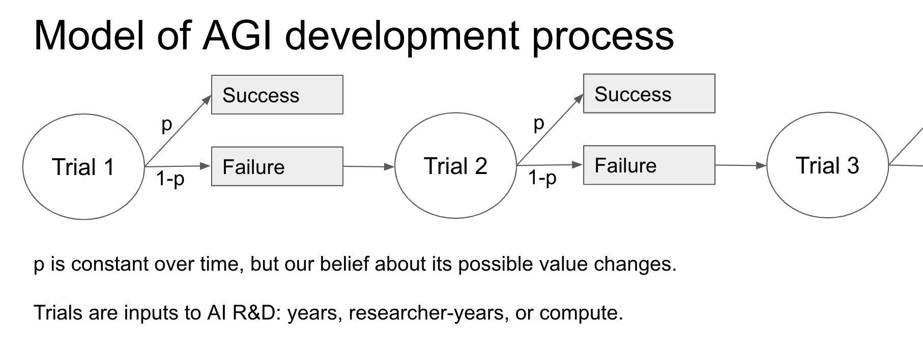
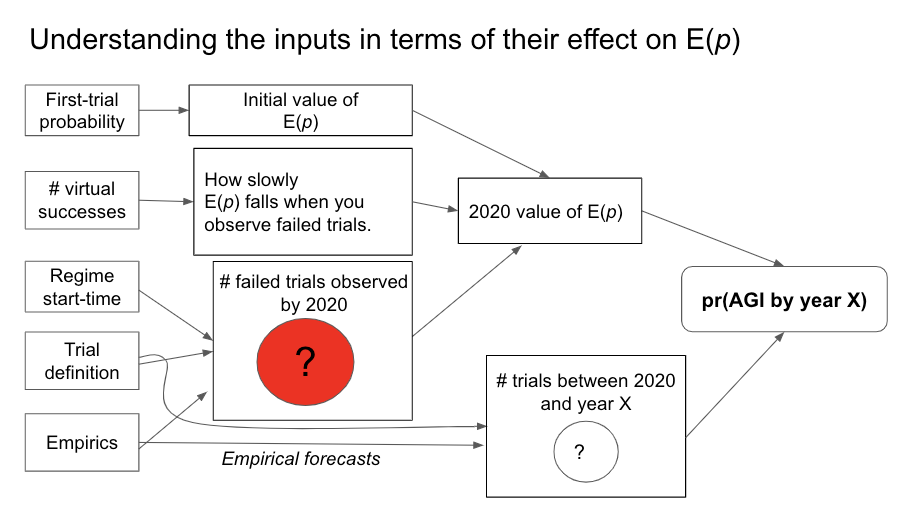
I find it useful to think about these inputs in terms of how E(p), our belief about the probability of success in the next trial, changes over time.27 The first-trial probability specifies the initial value of E(p) and the number of virtual successes describes how quickly E(p) falls when we observe failed trials.28 The regime start-time and trial definition determine how many failed trials we’ve observed to date; for some trial definitions (e.g. ‘one researcher-year’) we also need empirical data. The trial definition, perhaps in conjunction with empirical forecasts, also determines the number of trials that will occur in each future year. Together the four inputs determine a probability distribution over the year in which AGI will be developed. When the choice of inputs are informed by commonsense and relevant reference classes for AGI, I call such a distribution a semi-informative prior over AGI timelines.29 We will see that some highly subjective judgments seem to be needed to choose precise values for the inputs.

 

 

To use this framework to calculate pr(AGI by 2036) you need to choose values for each of the four inputs, estimate the number of trials that have occurred so far and estimate the number that will occur by 2036. I do this, and conduct various sensitivity analyses in Sections 4, 5 and 6. The rest of Section 3 explores the behavior of the semi-informative framework in more detail.

The following diagram gives a more detailed mathematical view of the framework:

 

 

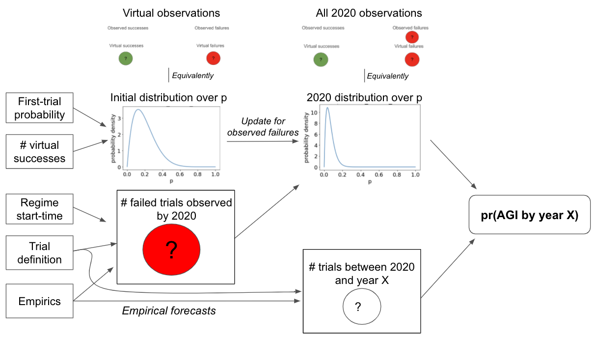
The first-trial probability and # virtual successes determine your initial probability distribution over p. This initial distribution corresponds to the number of virtual successes and virtual failures. The start-time and trial definition determine the number of observed failures by 2020. Updating on these failures creates you 2020 probability distribution over p. The 2020 distribution, together with the number of trials between 2020 and year X, determines pr(AGI by year X).]

3.2 The semi-informative priors framework can solve problems with using uninformative priors

This section identifies two problems with the application of Laplace’s rule of succession to AGI timelines, and argues that both can be addressed by the semi-informative priors framework.

3.2.1 Uninformative priors are aggressive about AGI timelines

Before the first trial, an uninformative prior implies that E(p) is 0.5.30 So our application of uninformative priors to AGI timelines implies that there was a 50% probability of developing in AGI in the first year of effort. Worse, it implies that there was a 91%31 probability of developing AGI in the first ten years of effort.32 The prior is so uninformative that it precludes the commonsense knowledge that highly ambitious R&D projects rarely succeed in the first year of effort!33

The fact that these priors are initially overly optimistic about the prospects of developing AGI means that, after updating on the failure to develop it so far, they will still be overly optimistic. For if we corrected their initial optimism by reducing the first-trial probability, the derived pr(AGI by 2036) will also decrease as a result. Their unreasonable initial optimism translates into unreasonable optimism about pr(AGI by 2036).

To look at this from another angle, when you use an uninformative prior the only source of skepticism that we’ll build AGI next year is the observed failures to date. But in reality, there are other reasons for skepticism: the bare fact that ambitious R&D projects typically take a long time means that the prior probability of success in any given year should be fairly low.

In the semi-informative priors framework, we can address this problem by choosing a lower value for the first-trial probability. In this framework there are two sources of skepticism that we’ll build AGI in the next trial: the failure to develop AGI to date and our initial belief that a given year of effort is unlikely to succeed.

3.2.2 The predictions of uninformative priors are sensitive to trivial changes in the trial definition

A further problem is that certain predictions about AGI timelines are overly sensitive to the trial definition. For example, if I had defined a trial as two years, rather than one, Laplace’s rule would have predicted a 83%34 probability of AGI in the first 10 years rather than 91%. If I had used one month, the probability would have been 99%.35 But predictions like these should not be so sensitive to trivial changes in the trial definition.36 Further, there doesn’t seem to be any privileged choice of trial definition in this setting.

This problem can be addressed by the semi-informative priors framework. We can use a procedure for choosing the first-trial probability that makes the framework’s predictions invariant under trivial changes in the trial definition. For example, we might choose the first-trial probability so that the probability of AGI in the first 20 years of effort is 10%. In this case, the model’s predictions will not materially change if we shift our trial definition from 1 year to (e.g.) 1 month: although there will be more trials in each period of time, the first-trial probability will be lower and these effects cancel.37

In fact, using common sense and analogous reference classes to select the first-trial probability naturally has this consequence. Indeed, all the methods of constraining the first-trial probability that I use in this report are robust to trivial changes in the trial definition.

3.3 How does the semi-informative priors framework behave?

There are a few features of this framework that it will be useful to keep in mind going forward.

• If your first-trial probability is smaller, your update from failure so far is smaller. If it takes 100 failures to reduce E(p) from 1/100 to 1/200, then it takes 200 failures to reduce E(p) from 1/200 to 1/400, holding the number of virtual successes fixed.38
• The first-trial probability is related to the median number of trials until success. Suppose your first-trial probability is 1/N and there’s 1 virtual success. Then, it turns out, the probability of success within the first (N – 1) trials is 50%.39
• E(p) is initially dominated by the first-trial probability; after observing many failures it’s dominated by your observed failures. Suppose your first-trial probability is 1/N and you have v virtual successes. After observing n failures, it turns out that E(p) = 1(N + n/v). For small values of n, E(p) is approximately equal to the first-trial probability. For large values of n, n/v ≫ N , E(p) is dominated by the update from observed failures.

3.4 Strengths and weaknesses

Here are some of the framework’s strengths:

• Quantifies the size of the negative update from failure so far. We can compare the initial value of E(p) with its value after updating on the failed trials observed so far. The ratio between these values quantifies the size of the negative update from failure so far.
• Highlights the role of intuitive parameters. The report’s analysis reveals the significance of the first-trial probability, regime start-time, the trial definition, and empirical assumptions for the bottom line. These are summarized in the conclusion.
• Arguably appropriate for expressing deep uncertainty about AGI timelines.
  • The framework produces a long-tailed distribution over the total time for AGI, reflecting the possibility that AGI will not be developed for a very long time (more here).
  • The framework can express Pareto distributions (more here), exponential distributions (more here), and uninformative priors as special cases.
  • The framework spreads probability mass fairly evenly over trials.40 For example, it couldn’t express the belief that AGI will probably be developed between 2050 and 2070, but not in the periods before or after this.
  • The framework avoids using anything like “I’m x% of the way to completing AGI” or “X of Y key steps on the path to AGI have been completed.” This is attractive if you believe I am not in a position to make more direct judgments about these things.

Here are some of the framework’s weaknesses:

• Incorporates limited kinds of evidence.
  • The framework excludes evidence relating to how close we are to AGI and how quickly we are getting there. For some, this is the most important evidence we have.
  • It excludes knowledge of an end-point, a time by which we will have probably developed AGI. So it cannot express (log-)uniform distributions (more here).
  • Evidence only includes the binary fact we haven’t developed AGI so far, and information from relevant reference classes about how hard AGI might be to develop.
• Near term predictions are too high. Today’s best AI systems are not nearly as capable as AGI, which should decrease our probability that AGI is developed in the next few years. But the framework doesn’t take this evidence into account.
• Insensitive to small changes in the definition of AGI. The methods I use to constrain the inputs to the framework involve subjective judgments about vague concepts. If I changed the definition of AGI to make it slightly easier/harder to achieve, the judgments might not be sensitive to these changes.
• Assumes a constant chance of success each trial. This is of course unrealistic; various factors could lead the chance of success to vary from trial to trial.
  • The assumption is more understandable given that the framework purposely excludes evidence relating to the details of the AI R&D process.
  • Appendix 12 argues that my results are driven by my choice of inputs to the framework, not by the framework itself. If this is right, then relaxing the problematic assumption would not significantly change my results.
  • Indeed, I analyzed sequential models in which multiple steps must be completed to develop AGI. pr(next trial succeeds) is very low in early years, rises to a peak, and then slowly declines. I compared my framework to a sequential model, with the inputs to both chosen in a similar way. Although pr(next trial succeeds) was initially much lower for the sequential model, after a few decades the models agreed within a factor of 2. The reason is that the sequential models are agnostic about how many steps still remain in 2020; for all they know just one step remains! Such agnostic sequential models have similar pr(AGI by year X) to my framework once enough time has passed that all the steps might have been completed. This is shown by the similar steepness of the lines.41
    

    

     

  • That said, the argument in Appendix 12 is not conclusive and I only analyzed a few possible types of sequential model. It is possible that other ways of constructing sequential models, and other approaches to outside view forecasting more generally, may give results that differ more significantly from my framework.

3.5 How do the inputs to the framework affect pr(AGI by 2036)?

How does pr(AGI by year X) depend on the inputs to the semi-informative priors framework? I did a sensitivity analysis around how varying each input within a reasonable range alters pr(AGI by 2036); the other inputs were left as in the initial Laplacian calculation.

The values in this table are not trustworthy because they use a first-trial probability of 0.5, which is much too high. I circle back and discuss each input’s effect on the bottom line in Section 8. Nonetheless, the table illustrates that the first-trial probability has the greatest potential to make the bottom line very low, and its uncertainty spans multiple orders of magnitude. This motivates an in-depth analysis of the first-trial probability in the next section.

 

INPUT	VALUES TESTED	RANGE FOR PR(AGI BY 2036)	COMMENTS
Regime start-time	1800 – industrial revolution 1954 – Dartmouth conference 2000 – brain-compute affordable (explained in Section 5)	[0.07, 0.43]	I discuss that even earlier regime start-times in Section 5. 0.43 corresponds to ‘2000’. When the first-trial probability is constrained within reasonable bounds, this range is much smaller.
Trial definition	A calendar year A researcher-year 1% increase in total researcher-years so far (See explanations of these definitions here)	[0.14, 0.71]	0.71 corresponds to ‘a researcher-year’ When the first-trial probability is constrained within reasonable bounds, this range is much smaller.
Number of virtual successes	0.5, 1	[0.11, 0.2]	I explain why I prefer the range [0.5, 1] for the case of AGI in Section 5.
First-trial probability	0.5, 0.1, 10-2, 10-3, 10-4	[1/1000, 0.2]

The next section, Section 4, discusses how we might constrain the first-trial probability for AGI; it also implicitly argues that it was reasonable for me to countenance such small values for first-trial probability in this sensitivity analysis. After this, Section 5 revisits the importance of the other inputs. Both Sections 4 and 5 assume that a trial is a calendar year; in Section 6 I consider other trial definitions.

4 Constraining the first-trial probability

The sensitivity analysis in the previous section suggested that the first-trial probability was the most important input for determining pr(AGI by 2036). This section explains my preferred methodology for choosing the first-trial probability (here) and then makes an initial attempt to put this methodology into practice in the case of AGI (here).

4.1 How to constrain the first-trial probability in principle

One compelling way to constrain the first-trial probability for a project’s duration would be as follows:

1. List different reference classes that seem potentially relevant to the project’s likely difficulty and duration. Each reference class will highlight different features of the project that might be relevant.
2. For each of these reference classes, try to constrain or estimate the first-trial probability using a mixture of data and intuitions. This leaves you with one constraint for each reference class. These constraints should be interpreted flexibly; they are merely suggestive and can be overridden by other considerations.
3. Weight each constraint by how relevant you think its reference class is to the project. Then, either by taking a formal weighted sum or by combining the individual constraints in an informal way, arrive at an all-things-considered constraint of the first-trial probability.

To illustrate this process, I’ll give a brief toy example with made-up numbers to show what these steps might look like when the project is developing AGI. To make the example short, I’ve removed most of the reasoning that would go into a comprehensive analysis, leaving only the bare bones.

1. List multiple different reference classes for the development of AGI:
   • ‘Hard computer science problem’ – the frequency with which such problems are solved is potentially relevant to the probability that developing AGI, an example of such a problem, is completed.
   • ‘Development of a new technology that leads to the automation of a wide range of tasks’ – the frequency at which such technologies are developed is potentially relevant to the probability that AGI, an example of such a technology, is developed.
   • ‘Ambitious milestone that an academic STEM field is trying to achieve’ – the time it typically takes for such fields to succeed is potentially relevant to the probability that the field of AI R&D will succeed.
2. Constrain the first-trial probability for each reference classes:
   • Data about hard computer science problems suggests about 25% of such problems are solved after 20 years of effort. (These numbers are made up.) On the basis of this reference class, we should choose AGI’s first-trial probability so that the chance of success in the first 20 years is close to 25%. This corresponds to a first-trial probability of 1/61. So this reference class suggests that the first-trial probability be close to 1/60.
   • Data about historical technological developments suggest that developments with an impact on automation comparable to AGI occur on average less often than once each century.42 So our probability that such a development occurs in a given year should be less than 1%. On the basis of this reference class, we should choose AGI’s first-trial probability so that the chance of success each year is <1%. So this reference class suggests that the first-trial probability be <1/100.
   • Data about whether STEM fields achieve ambitious milestones they’re trying to achieve seems to suggest it is not that rare for fields to succeed after only a few decades of sustained effort. On the basis of this reference class, we should choose AGI’s first-trial probability so that the chance of success in the first 50 years is >5%. This implies first-trial probability ≫1/950. So consideration of this reference class suggests that the first-trial probability should be >1/1000.
3. To reach an all-things-considered view on AGI’s first-trial probability, weigh each constraint by how relevant you think the associated reference class is to the likely difficulty and duration of developing AGI. For example, someone might think the latter two classes are both somewhat relevant but put less weight on “hard computer science problem” because they think AGI is more like a large collection of such problems than any one such problem. As a consequence, their all things-considered view might be that AGI’s first-trial probability should be >1/1000 and <1/100.

This is just a brief toy example (again, with made-up numbers) to illustrate what my preferred process for constraining the first-trial probability might look like. Clearly, difficult and debatable judgment calls must be made in all three steps. In the first step, a short list of relevant reference classes must be identified. In the second step, data about the reference class must be interpreted to derive a constraint for the first-trial probability. In the third step, judgment calls must be made about the relevance of each reference class and the individual constraints must be combined together.

It may be that no reference class both has high quality data and is highly relevant to the likely duration of developing AGI. In this case, my preference is to make the most of the reference classes and data that is available, interpreting the derived constraints as no more than suggestive. It may be that by making many weak arguments, each with a different reference class, we can still obtain a meaningful constraint on our all-things-considered first-trial probability. Even if we do not put much weight in any particular argument, multiple arguments collectively may help us triangulate what values for the first-trial probability are reasonable.

4.2 Constraining AGI’s first-trial probability in practice

The first-trial probability should of course depend on the trial definition. For example, the first-trial probability should be higher if a trial is ‘5 calendar years’ than if it’s ‘1 calendar year’; it should be different again if a trial is ‘a researcher-year’. In this section I assume that a trial is ‘one calendar year of sustained AI R&D effort’,43 which I abbreviate to ‘1 calendar year’. I also assume that the regime start-time is 1956 and the number of virtual successes is 1; I consider the effects of varying these inputs in the next section.

The focus of this project has been in the articulation of the semi-informative priors framework, rather than in finding data relevant for constraining the first-trial probability. As such, I think all of the arguments I use to constrain the first-trial probability are fairly weak. In each case, either the relevance of the reference class is unclear, I have not found high quality data for the reference class, or both. Nonetheless, I have done my best to use readily available evidence to constrain my first-trial probability for AGI, and believe doing this has made my preferred range more reasonable.

I currently favor values for AGI’s first-trial probability in the range [1/1000, 1/100], and my central estimate is 1/300.

This preferred range is informed by four reference classes. In each case, I use the reference class to argue for some constraint on, or estimate of, the first-trial probability. The four reference classes were not chosen because they are the most relevant reference classes to AGI, but because I was able to use them to construct constraints for AGI’s first-trial probability that I find somewhat meaningful. While I extract inequalities or point estimates of the first-trial probability from each reference class, my exact numbers shouldn’t be taken seriously and I think one could reasonably differ by at least a factor of 3 in either direction, perhaps more. Further, people might reasonably disagree with my views on the relevance of each reference class.

I explain my thinking about each reference class in detail in supplementary documents that are linked individually in the table below. These supplementary documents are designed to help the reader use their own beliefs and intuitions to derive a constraint from each reference class. I encourage readers use these to construct their own constraints for AGI’s first-trial probability. Much more work could be done finding and analyzing data to better triangulate the first-trial probability, and I’d be excited about such work being done.

The following table summarizes how the four reference classes inform my preferred range for the first-trial probability. Please keep in mind that I think all of these arguments are fairly weak and see all the constraints and point estimates as merely suggestive.

REFERENCE CLASS	ARGUMENT DERIVING A CONSTRAINT ON THE FIRST-TRIAL PROBABILITY (FTP)	CONSTRAINTS AND ESTIMATES OF FTP	MY VIEW ON THE INFORMATIVENESS OF THIS REFERENCE CLASS
Ambitious but feasible technology that a serious STEM field is explicitly trying to develop (see more).	Scientific and technological R&D efforts have an excellent track record of success. Very significant advances have been made in central and diverse areas of human understanding and technology: physics, chemistry, biology, medicine, transportation, communication, information, and energy. I list 11 examples, with a median completion time of 75 years. Experts regard AGI as feasible in principle. Multiple well-funded and prestigious organizations are explicitly trying to develop AGI. Given the above, we shouldn’t assign a very low probability to the serious STEM field of AI R&D achieving one of its central aims after 100 years of sustained effort.	Lower bound: ftp > 1/3000 – pr(AGI within 100 years of effort) >3%, or pr(AGI within 30 years of effort) >1%. Conservative estimate: ftp = 1/300 – pr(AGI within 100 years of effort) = 25%. Optimistic estimate: ftp = 1/50 – pr(AGI within 50 years of effort) = 50%.	In my view, this is the most relevant reference class of the four that I consider. The fact that a serious STEM field is trying to build AGI is clearly relevant to AGI’s probability of being developed. That said, STEM fields vary in their degree of success and AGI may be an especially ambitious technology, reducing the relevance of this reference class. There is also a selection bias in the list of successful STEM fields (that I try to adjust for in the conservative estimate).
Possible future technology that a STEM field is trying to build in 2020 (see more).	This report focuses on AGI and its core reason for having a non-tiny first-trial probability is that a STEM field is trying to build AGI. But we could apply the same framework to multiple different technologies that STEM fields are trying to build in 2020. It would be worrying if, by doing this many times, we could deduce that the expected number of transformative technologies that will be developed in a 10 year period is very large. We can avoid this problem by placing an upper bound on the first-trial probability.	Conservative upper bound: ftp < 1/100 – STEM fields are trying to build 10 transformative technologies in 2020, but I expect < 0.5 technologies to be developed in a ten year period). Aggressive upper bound: fpt < 1/300 – As above but expect <0.25 to be developed.	In principle, I think this reference class is highly relevant. We shouldn’t trust this methodology if applying it elsewhere leads to unrealistic predictions. In practice, however, it’s hard to make this objection cleanly for various reasons. As such, I put very little stock in the precise numbers derived. I’m unsure what constraint a more comprehensive analysis would suggest.
Technological development that has a transformative effect on the nature of work and society (see more).	Some people believe that AGI would have a transformative effect on the nature of work and society. We can use the history of technological developments to estimate the frequency with which transformative developments like AGI occur. This frequency should guide the probability ptransf I assign to a transformative development occurring in a given year. My annual probability that AGI is developed should be lower than ptransf, as it’s less likely that AGI in particular is developed than that any transformative development occurs.	Upper bound: ftp < 1/130 – Assume two transformative events have occurred. Assume the probability of a transformative development occurring in a year is proportional to the amount of technological progress in that year.	I believe that a technology’s impact is relevant to the likely difficulty of developing it (see more). So I find this reference class somewhat informative. Further, a common objection to AGI is that it would have such a large impact so is unrealistic. This reference class translates this objection into a constraint on the ftp. However, there are very few (possibly zero) examples of developments with impact comparable to AGI; this makes this reference class less informative.
Notable mathematical conjectures (see more).	AI Impacts investigated how long notable mathematical conjectures, not explicitly selected for difficulty, take to be resolved. They found that the probability that an unsolved conjecture is solved in the next year of research is ~1/170.	ftp ~ 1/170	The data for this reference class is better than for any other. However, I doubt that resolving a mathematical conjecture is similar to developing AGI. So I view this as the least informative reference class.

The following table succinctly summarizes the most relevant inputs for forming an all-things-considered view.

 

REFERENCE CLASS	CONSTRAINTS AND POINT ESTIMATES OF THE FIRST-TRIAL PROBABILITY (FTP)	INFORMATIVENESS
Ambitious but feasible technology that a serious STEM field is explicitly trying to build (see more).	Lower bound: ftp > 1/3000 Conservative estimate: ftp ~ 1/300 Optimistic estimate: ftp ~ 1/50	Most informative.
High impact technology that a serious STEM field is trying to build in 2020 (see more).	Conservative upper bound: ftp < 1/100 Aggressive upper bound: fpt < 1/300	Weakly informative.
Technological development that has a transformative effect on the nature of work and society (see more).	Upper bound: ftp < 1/130	Somewhat informative.
Notable mathematical conjectures (see more).	ftp ~ 1/170	Least informative.

I did not find it useful to use a precise formula to combine the constraints and point estimates from these four reference classes. Overall, I favor a first-trial probability in the range [1/1000, 1/100], with a preference for the higher end of that range.44 If I had to pick a number I’d go with ~1/300, perhaps higher.

The numbers I’ve derived depend on subjective choices about which references classes to use (reviewers suggested alternatives45), how to interpret them (the reference classes are somewhat vague46), and how relevant they are to AGI. I did my best to use a balanced range of reference classes that could drive high and low values. These subjective judgments would probably not be sensitive to small changes in the definition of AGI (see more).

The following table shows how different first-trial probabilities affect the bottom line, assuming that 1 virtual success and a regime start-time of 1956.47

FIRST-TRIAL PROBABILITY	PR(AGI BY 2036)
1/50	12%
1/100	8.9%
1/200	5.7%
1/300	4.2%
1/500	2.8%
1/1000	1.5%
1/2000	0.77%
1/3000	0.52%

(Throughout this report, I typically give results to 2 significant figures as it is sometimes useful for understanding a table. However, I don’t think precision beyond 1 significant figure is meaningful.)

Based on the table and my preferred range for the first-trial probability, my preferred range for pr(AGI by 2036) is 1.5 – 9%, with my best guess around 4%. I will be refining this preferred range over the course of the report. (At each time, I’ll refer to the currently most refined estimate as my “preferred range,” though it may continue to change throughout the report.)

5 Importance of other inputs

The semi-informative priors framework has four inputs:

• Regime start-time
• Trial definition
• Number of virtual successes
• First-trial probability

In the previous section we assumed that the regime start-time was 1956, the number of virtual successes was 1, and the trial definition was a ‘calendar year’. I then suggested that a reasonable first-trial probability for AGI should probably be in the range [1/1000, 1/100]. This corresponded to a bottom line pr(AGI by 2020) in the range [1.5%, 9%].

In this section, I investigate how this bottom line changes if we allow the regime start-time and the number of virtual successes to vary within reasonable bounds, still using the trial definition ‘calendar year’. My conclusion is that these two inputs don’t affect the bottom line much if your first-trial probability is below 1/100. They matter even less if your first-trial probability is below 1/300. The core reason for this is that if your first-trial probability is lower, you update less from observed failures. Both the regime start-time and the number of virtual successes affect the size of the update from observed failures; if this update is very small to begin with (due to a low first-trial probability), then these inputs make little difference.

Overall, this section slightly widens my preferred range to [1%, 10%]. If this seems reasonable, I suggest skipping to Section 6.

The section has three parts:

• I briefly explain with an example why having a lower first-trial probability means that you update less from observed failures (here).
• I investigate how the number of virtual successes affects the bottom line (here).
• I investigate how the regime start-time affects the bottom line (here).

5.1 The lower the first-trial probability, the smaller the update from observing failure

To illustrate this core idea, let’s consider a simple example:

You’ve just landed in foreign land that you know little about and are wondering about the probability p that it rains each day in your new location. You’ve been there 10 days and it hasn’t rained yet.

Let’s assume each day is a trial and use 1 virtual success. Ten failed trials have happened. We’ll compare the size of the update from these failures for different possible first-trial probabilities.

If your first-trial probability was 1/2, then your posterior probability that it rains each day is E(p) = 1/(2 + 10) = 1/12 (see formula in Section 3.3). You update E(p) from 1/2 to 1/12.

But if your first-trial is 1/50 – you initially believed it was very unlikely to rain on a given day – then your posterior is E(p) = 1/(50 + 10) = 1/60. You update E(p) from 1/50 to 1/60. This is a smaller change in your belief about the probability that it rains , both in absolute and percentage terms.48

A similar principle is important for this section. If you have a sufficiently low first-trial probability that AGI will be developed, then the update from failure to develop it so far will make only a small difference to your probability that AGI is developed in future years. Changing the number of virtual successes and the regime start-time changes the exact size of this update; but if the update is small then this makes little difference to the bottom line.

5.2 Number of virtual successes

In this section I:

• Discuss the meaning of the number of virtual successes (here).
• Explain what I range I prefer for this parameter (here).
• Analyze the effect of varying this parameter on the bottom line (here).

5.2.1 What is the significance of the number of virtual successes?

Recall that, in this model, p is the constant probability of developing AGI in each trial. Intuitively, p represents the difficulty of developing AGI. I am unsure about the true value of p so place a probability distribution – a beta distribution, in fact – over its value. E(p) is our expected value of p, our overall belief about how likely AGI is to be developed in one trial, given the outcomes (failures) in any previous trials.

The number of virtual successes, together with the first-trial probability, determines your initial probability distribution over p. The following graphs show this initial distribution for different values of these two inputs, which I shorten to nvs and ftp on the graph labels.

 

 

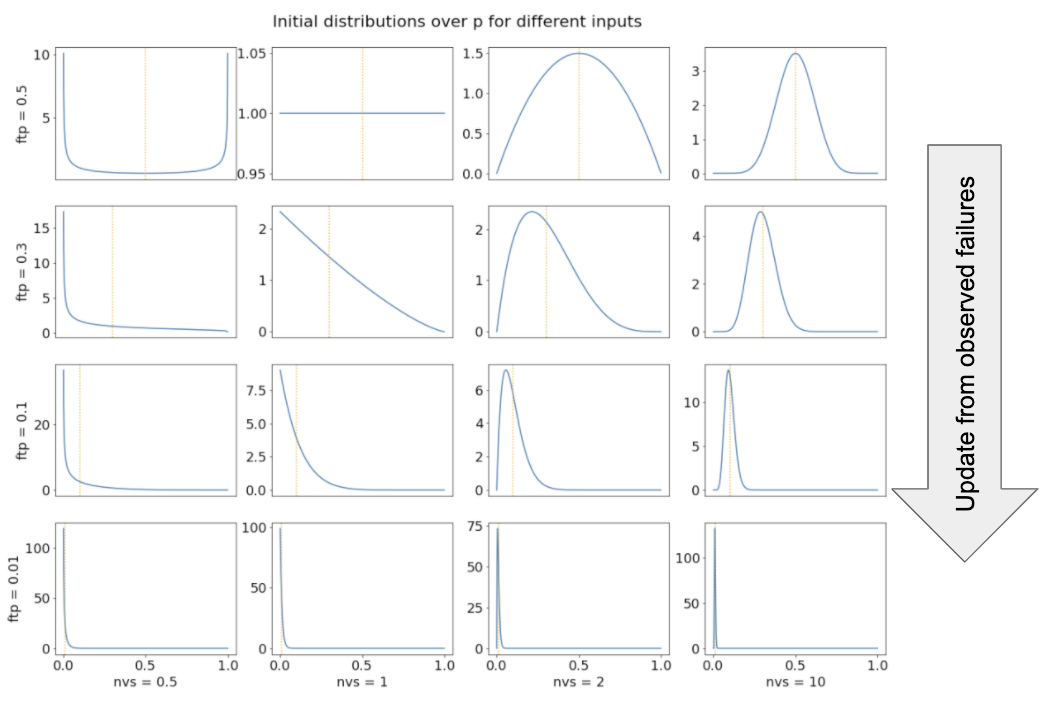
The vertical orange dotted lines shows the value of the first-trial probability. More virtual successes makes the distribution spike more sharply near the first-trial probability; this represents increased confidence about how difficult AGI is to develop. Conversely, fewer virtual successes spreads out probability mass towards extremal values of p; this represents more uncertainty about the difficulty of developing AGI. In other words, the number of virtual successes relates to the variance of our initial estimate of p. More virtual successes → less variance.

We can relate this to the reference classes discussed in Section 4. If there is a strong link between AGI and one particular reference class, and items in that reference class are similarly difficult to one other, this suggests we can be confident about how difficult AGI will be. This would point towards using more virtual successes. Conversely, if there are possible links to multiple reference classes, these reference classes differ from each other in their average difficulty, and the items within each reference class vary in their difficulty, this suggests we should be uncertain about how difficult AGI will be. This would point towards using fewer virtual successes.49

As discussed in Section 3, fewer virtual successes means that E(p) changes more when you observe failed trials (holding ftp fixed). So we can think of virtual successes as representing the degree of resiliency of our belief about p. An alternative measure of resiliency would be the total number of virtual observations: virtual successes + virtual failures. I explain why I don’t use this measure in an appendix.

We can also use the above graphs to visualize what happens to our distribution over p when we observe failed trials. The distribution changes just as if we had decreased the first-trial probability.50 If our initial distribution is one of the top graphs then as we observe failures it will morph into the distributions shown directly below it.51

5.2.2 What is a reasonable range for the number of virtual successes?

This section briefly discusses a few ways to inform your choice of this parameter.

I favor values for this parameter in the range [0.5, 1], and think there are good reasons to avoid values as high as 10 or as low as 0.1.

5.2.2.1 Eyeballing the graphs

One way to inform your choice of number of virtual successes is to eyeball the above collection of graphs, and favor the distributions that look more reasonable to you. For example, I prefer the probability density to increase as p approaches 0 – e.g. I think p is more likely to be between 0 and 1 / 10,000 than between 1 / 10,000 and 2 / 10,000. This implies that the number of virtual successes ≤ 1.52

Such considerations aren’t very persuasive to me, but I give them some weight.

5.2.2.2 Consider what a reasonable update would be

Suppose your first-trial probability for AGI is 1/100. That means that initially you think a year of research has a 1/100 chance of successfully developing AGI: E(p) = 1/100. Suppose you then learn that 50 years of research have failed to produce AGI. Later, you learn that a further 50 years have again failed. The following table shows your posterior value of E(p) after these updates.53

NUMBER OF VIRTUAL SUCCESSES	0.1	0.5	1	2	10
Initial E(p)	1/100	1/100	1/100	1/100	1/100
E(p) after 50 failures	1/600	1/200	1/150	1/125	1/105
E(p) after 100 failures	1/1100	1/300	1/200	1/150	1/110

I recommend choosing your preferred number of virtual successes by considering which update you find the most reasonable. I explain my thinking about this below.

Intuitively, I find the update much too large with 0.1 virtual successes. If you initially thought the annual chance of developing AGI was 1/100, 50 years of failure is not that surprising and it should not reduce your estimate down as low as 1/600.54 Such a large update might be reasonable if we initially knew that AGI would either be very easy to develop, or it would be very hard. But, at least given the evidence this project is taking into account, we don’t know this.

Similarly, I intuitively find the update with 10 virtual successes much too small. If you initially thought the annual chance of developing AGI was 1/100, then 100 years of failure is somewhat surprising (~37%) and should reduce your estimate down further than just to 1/110.55 Such a small update might be reasonable if we initially had reason to be very confident about exactly how hard AGI would be to develop (e.g. because we had lots of very similar examples to inform our view). But this doesn’t seem to be the case.

I personally find the updates most reasonable when the number of successes is 1, followed by those for 0.5. This and the previous section explains my preference for the range [0.5, 1]. I expect readers to differ somewhat, but would be surprised if people preferred values far outside the range [0.5, 2].

5.2.2.3 A pragmatic reason to prefer number of virtual successes = 1

The mathematical interpretation of the first-trial probability is easier to think about if there is 1 virtual success.

In this case, if the first-trial probability = 1 / N then it turns out that there’s a 50% chance of success within the first N – 1 trials. This makes it easy to translate claims about the first-trial probability into claims about the median expected time until success. This isn’t true for other numbers of virtual successes.

This consideration could potentially be a tiebreaker.

5.2.3 How does varying the number of virtual successes affect the bottom line?

The following table shows pr(AGI by 2036) for different numbers of virtual successes and first-trial probabilities. I use a regime start-time of 1956.

NUMBER OF VIRTUAL SUCCESSES	FIRST-TRIAL PROBABILITY
	1/100	1/300	1/1000
0.1	2.0%	1.6%	0.93%
0.25	4.1%	2.7%	1.2%
0.5	6.4%	3.6%	1.4%
1	8.9%	4.2%	1.5%
2	11%	4.7%	1.5%
4	13%	4.9%	1.6%
10	14%	5.1%	1.6%

There are a few things worth noting:

• Fewer virtual successes means a lower pr(AGI by 2036) as you update more from failures to date.
• Varying the number of virtual successes within my preferred range [0.5, 1] makes little difference to the bottom line.
• Varying the number of virtual successes makes less difference when the first-trial probability is lower.56
• Using very large values for the number of virtual successes won’t affect your bottom line much, but using very small values will.57 For example, the increase from 4 to 10 has very little effect, while the decrease from 0.25 to 0.1 has a moderate effect.

In fact, the above table may overestimate the importance of the number of virtual successes. This is because using fewer virtual successes may lead you to favor a larger first-trial probability, and these effects partially cancel out.

In particular, when choosing the first-trial probability one useful tool is to constrain or estimate the cumulative probability of success within some period. A smaller number of virtual successes will lower this cumulative probability, so you will need a larger first-trial probability in order to satisfy any given constraint.

	0.5 VIRTUAL SUCCESSES				1 VIRTUAL SUCCESS
First-trial probability	1/50	1/100	1/300	1/1000	1/100	1/300	1/1000
pr(AGI in first 50 years)	43%	30%	13%	4.7%	34%	14%	4.8%
pr(AGI in first 100 years)	56%	43%	23%	8.7%	50%	25%	9.1%
pr(AGI by 2036 | no AGI by 2020)	8.0%	6.4%	3.6%	1.4%	8.9%	4.2%	1.5%

For example, suppose you constrain the probability of success in the first 100 years of research to be roughly 50%. If you use 1 virtual success, your first-trial probability will be close to 1/100; but if you use 0.5 virtual successes, your first-trial probability will be closer to 1/50. As a consequence, using 0.5 virtual successes rather than 1 only decreases pr(AGI by 2036) by about 8.9% – 8.0% = 0.9%, rather than the 8.9% – 6.4% = 2.5% that it would be if you kept the first-trial probability constant.

(Using a table like this is in fact another way to inform your preferred number of virtual successes. Keeping the reference classes discussed in Section 4 in mind, you can decide which combination of inputs give the most plausible values for pr(AGI in first 50 years) and pr(AGI in first 100 years).)

Summary – How does varying the number of virtual successes affect the bottom line?

I prefer a range for the number of virtual successes of [0.5, 1]. If the first-trial probability ≤ 1/300, changes with this range make <1% difference to the bottom line; if the first-trial probability is as high as 1/100, changes in this range make <2% difference to the bottom line.58 Throughout the rest of the document, I use 1 virtual success unless I specify otherwise.

Note: the number of virtual successes has an increasingly large effect on pr(AGI by year X) for later years. Moving from 1 to 0.5 virtual successes reduces pr(AGI by 100) from 33% to 23% when first-trial probability = 1/100.

5.3 Regime start time

The regime start time is a time such that the failure to develop AGI before that time tells us very little about the probability of success after that time. Its significance in the semi-informative priors framework is that we update our belief about p – the difficulty of developing AGI – based on failed trials after the regime start time but not before it.

A natural choice of regime start time is 1956, the year when the field of AI R&D is commonly taken to have begun. However, there are other possible choices:

• 2000, roughly the time when an amount of computational power that’s comparable with the brain first became affordable.59
• 1945, the date of the first digital computer.
• 1650, roughly the time when classical philosophers started trying to represent rational thought as a symbolic system.

What about even earlier regime start times? Someone could argue:

Humans have been trying to automate parts of their work since society began. AGI would allow all human work to be automated. So people have always been trying to do the same thing AI R&D is trying to do. A better start-time would be 5000 BC.

The following table shows the bottom line for various values of the first-trial probability and the regime start-time.

PR(AGI BY 2036) FOR DIFFERENT INPUTS
	REGIME START-TIME
First-trial probability	2000	1956	1945	1650	5000 BC
1/50	19%	12%	11%	3.7%	0.23%
1/100	12%	8.9%	8.4%	3.3%	0.22%
1/300	4.8%	4.2%	4.1%	2.3%	0.22%
1/1000	1.5%	1.5%	1.5%	1.2%	0.20%

A few things are worth noting:

• If your first-trial probability is lower, changes in the regime start time make less difference to the bottom line.
• The highest values of pr(AGI by 2036) correspond to large first-trial probabilities and late regime start-times.
• Very early regime start-times drive very low pr(AGI by 2036) no matter what your first-trial probability.

However this last conclusion is misleading. The above analysis ignores the fact that the world is changing much more quickly now than in ancient times. In particular, technological progress is much faster.60 As a result, even if we take very early regime start-times seriously, we should judge that the annual probability of creating AGI is higher now than in ancient times. But my above analysis implicitly assumes that the annual probability p of success was the same in modern times as in ancient times. As a consequence, its update from the failure to build AGI in ancient times was too strong.

In response to this problem we should down-weight the number of trials occurring each year in ancient times relative to modern times. There are a few ways to do this:

• Weight each year by the global population in that year. The idea here is that twice as many people should make twice as much technological progress.
• Weight each year by the amount of economic growth that occurs in each year, measured as the percentage increase in Gross World Product (GWP). Though GWP is hard to measure in ancient times, economic growth is a better indicator of technological progress than the population.
• Weight each year by the amount of technological progress in frontier countries, operationalized as the percentage increase in French GDP per capita.61

As we go down this list, the quantity used to weight each year becomes more relevant to our analysis but our measurement of the quantity becomes more uncertain. I will present results for all three, and encourage readers to use whichever they think is most reasonable.

Each of these approaches assigns a weight to each year. I normalize the weights for each approach by setting the average weight of 1956-2020 to 1 – this matches our previous assumption of one trial per calendar year since 1956. Then I use the weights to calculate the number of trials before 1956. The following table shows the results when the regime start-time is 5,000 BC.

	APPROACH TO WEIGHTING EACH YEAR
	POPULATION	ECONOMIC GROWTH (%)	TECHNOLOGICAL PROGRESS (%)	ZERO WEIGHT BEFORE 195662
Trials between 5000 BC and 1956	168	220	139	0
First-trial probability	Pr(AGI by 2036)
1/2	6.4%	5.3%	7.3%	20%
1/100	4.6%	4.0%	5.0%	8.9%
1/300	2.9%	2.7%	3.1%	4.2%
1/1000	1.3%	1.2%	1.3%	1.5%

All three approaches to weighting each year give broadly similar results. They imply that a few hundred trials occurred before 1956, rather than thousands, and so pr(AGI by 2036) is only moderately down-weighted. The effect, compared with a regime start-time of 1956, is to push the bottom line down into the 1 – 7% range regardless of your first-trial probability.63 So if you regard very early regime start-times as plausible, this gives you a reason to avoid the upper-end of my preferred range of 1 – 9%.64

Summary – How does varying the regime start-time affect the bottom line?

Overall, the effect of very early regime start-times is to bring down the bottom line into the range 1 – 7% even if you have a very large first-trial probability. Late regime start-times would somewhat increase the higher end of my preferred range, potentially from 9 to 12%.

5.4 Summary – importance of other inputs

In Section 4 we assumed that there was 1 virtual success and that the regime start-time was 1956. On this basis my preferred range for pr(AGI by 2036) was 1.5 – 9%.

This basic picture changes surprisingly little when we consider different values for the number of virtual successes and the regime start-time.

• If your bottom line was towards the top of that range, then fewer virtual successes or an earlier regime-start time can push you slightly towards the bottom of that range. Conversely, a late regime start-time could raise your bottom line slightly.
• But if you were already near the bottom of that range, then varying these two inputs has very little effect. This is because when your first-trial probability is lower, you update less from the failure to develop AGI to date.

On this basis, my preferred range for pr(AGI by 2036) is now 1 – 10%,65 and my central estimate is still around 4%.66

All the analysis so far assumes that a trial is a calendar year. The next section considers other trial definitions.

6 Other trial definitions

Sections 4 and 5 applied the semi-informative priors methodology to the question of when AGI might be developed, assuming that a trial was ‘one calendar year of sustained AI R&D effort’. My preferred range for pr(AGI by 2036) was 1-10%, and my central estimate was about 4%.

This section considers trials defined in terms of the researcher-years and compute used in AI R&D. The resultant semi-informative priors give us AGI timelines that are sensitive to how these R&D inputs change over time.

When defining trials in terms of researcher-years, my preferred range shifts up to 2 – 15%, and my central estimate to 8%. When defining trials in terms of training compute, my preferred range shifts to 2 – 25% and my central estimate to 15% (though this is partly because a late regime start-time makes more sense in this context).

As before, I initially use 1 virtual success and a regime start time of 1956, and then revisit the consequences of relaxing these assumptions later.

6.1 Researcher-year trial definitions

In this section I:

• Describe my preferred trial definition relating to researcher-years (here).
• Discuss one way of choosing the first-trial probability for this definition, and its results for AGI timelines (here).

6.1.1 What trial definition do I prefer?

My preferred trial definition is ‘a 1% increase in the total researcher-years so far’.67 The semi-informative priors framework then assumes that every such increase has a constant but unknown chance of creating AGI.68

I can explain the meaning of this choice by reference to a popular economic model of research-based technological progress, introduced by Jones (1995):69

\( \dot A=δL_AA^ϕ \)

In our case A is the level of AI technological development, Ȧ ≡ dA/dt is the rate of increase of A,70 L_A is the number of AI researchers at a given time and δ is a constant.71 If φ > 0, previous progress raises the productivity of subsequent research efforts. If φ < 0, the reverse is true – perhaps because ideas become increasingly hard to find.

With this R&D model, my preferred trial definition can be deduced from two additional claims:

• φ < 1.
  • If this isn’t true, increasing L_A will increase the growth rate g_A. But evidence from 20th century R&D efforts consistently shows exponentially increasing L_A occurring alongside roughly constant g_A (see e.g. Bloom (2017) and Vollrath (2019) chapter 4). On this basis, Jones (1995) argues for restricting φ < 1.
• Each 1% increase in A has a constant probability of leading to the development of AGI.
  • This is not a trivial claim; a simple alternative would be to say that each absolute increase in A has a constant (prior) probability of leading to AGI.
  • This claim embodies the belief that our uncertainty about the number of researcher-years and the increase in A required to develop AGI spans multiple orders of magnitude.
  • It also reflects the idea that each successive 1% increase in the level of technology involves a similar amount of qualitative progress.

These two claims, together with the R&D model, imply that each successive 1% increase in total researchers years has a constant (unknown) probability of leading to AGI (proof in this appendix). With my preferred trial definition, the semi-informative priors framework makes exactly this assumption.

This definition has the consequence that if the number of AI researchers grows at a constant exponential rate72 then the number of trials occurring each year is constant.73 In this sense, the trial definition is a natural extension of ‘a calendar year’. Of course, the faster the growth rate, the more trials occur each year.

I investigated two other trial definitions relating to researcher-years, each with a differing view on the marginal returns of additional research. I discuss them in this appendixand explain why I don’t favor the alternatives.

6.1.2 Choosing the first-trial probability for the researcher-year trial definition

To calculate pr(AGI by 2036) with this trial definition, we must constrain the first-trial probability. To avoid confusion, let ftp_cal refer to the first-trial probability when a trial is ‘a calendar year’ and let ftp_res refer to the first-trial probability when a trial is ‘a 1% increase in the total researcher-years so far’.

One possible way to choose ftp_res would be to look at data on how many researcher-years is typically required to achieve ambitious technological milestones. This section pursues another strategy: deriving ftp_res from ftp_cal.

When choosing ftp_cal in Section 4, we assumed that there was a sustained R&D effort from a serious academic field but we did not consider exactly how large that effort was. For ftp_res, I wish to take into account exactly how quickly the field of AI R&D is growing. Here’s the intuitive idea behind my proposal for choosing ftp_res:

If the growth of AI R&D is typical of R&D fields, then moving from the ‘calendar year’ trial definition to this new ‘researcher-year’ trial definition shouldn’t change our quantitative predictions pr(AGI by year X).

In addition, if the growth of AI R&D is surprisingly fast (/slow), then we should adjust the probability of developing AGI up (/down) compared to the ‘calendar year’ trial definition. This idea is used as the basis for deriving ftp_res from ftp_cal.

My proposal for calculating ftp_res is as follows. First, identify a growth rate, g_exp, such that if the total researcher-years grew at gexp, we would regard the probabilities from the ‘calendar year’ trial definition as reasonable. Roughly speaking, g_exp is how fast we (implicitly) expected the number of researcher-years in AI R&D to grow when we were still using the trial definition ‘a calendar year’. g_exp should be based on empirical data about the typical growth of R&D fields; ideally it would be the average growth rate of the R&D efforts I used to inform my estimate of ftp_cal in Section 4. This first step selects g_exp.

Second, choose ftp_res so that, on the assumption that AI researcher-years are growing at g_exp, pr(AGI by year X) is the same as for the ‘calendar year’ trial definition. In this way I calculate ftp_res from ftp_cal and g_exp.74

To calculate pr(AGI by 2036), we must estimate the number of failed trials in 1956 – 2020 and the number of additional trials occurring in 2020 – 2036. To this end, I make an assumption about the actual growth rate of AI researcher-years, g_act. (For simplicity, this analysis assumes both g_act and g_exp to be constant.) We can use g_act to calculate the number of trials that occur in each year. As before, we update our prior based on the failed trials before 2020 and then calculate pr(AGI by 2036) based on the trials that will occur in 2020-2036.

 

 

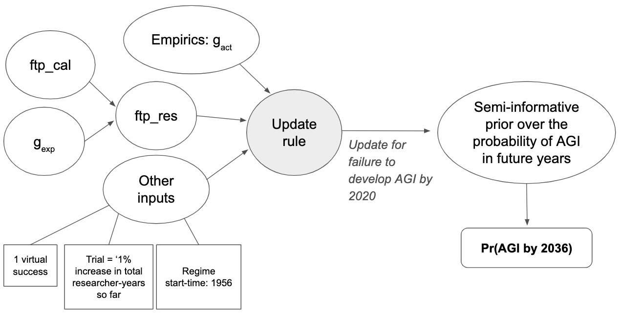
If g_act = g_exp – the growth of AI R&D is typical – then the AGI timelines from this method are identical to when a trial was a ‘calendar year’. Indeed, I chose ftp_res so that this would be true. If g_act > g_exp, more trials occur each year and the probability of AGI is higher.75 Conversely, if g_act < g_exp the probability is lower. So this method adjusts up or down from when a trial was a ‘calendar year’ depending on whether AI R&D growth is surprisingly big or small.

How should we choose g_exp? The growth rates of different STEM fields are highly heterogeneous (see tables 2 – 4 in Bloom (2017)), so any choice is somewhat arbitrary. For this analysis, I primarily use g_exp = 4.3%. This is the average growth of the effective number of researchers in US R&D from 1930 to 2014 (see Bloom (2017)). If AI R&D had stayed a constant fraction of overall US R&D, it would have grown at 4.3%. This is a reasonable candidate for g_exp, though higher values could be argued for.76 I also show results for g_exp = 8.6% in an appendix, the high-end of the growth rates of individual fields in Bloom (2017).

How should we choose g_act? Ideally, it would equal the average growth rate in the number of AI researchers (ideally controlling for their quality). Unfortunately, none of the data sources that I’ve reviewed report this statistic directly. They report the number of researchers at a particular time, increases in conference attendance and increases in research papers. The values for g_act that these sources suggest range from 3% to 21%. My preferred source is the AI Index 2019, which finds that the number of peer-reviewed papers has grown by 11.4% on average over the last 20 years.

The following tables show the bottom line for different choices of ftp_cal and g_act. For each ftp_cal, the table also shows pr(AGI by 2036) when a trial is a calendar year. The table assumes g_exp = 4.3%, I show the analogous table for g_exp = 8.6% in this appendix. (I’ve highlighted the inputs and output for my central estimate in bold.)

GEXP = 4.3%		PR(AGI BY 2036)
		CALENDAR YEAR TRIAL DEFINITION	RESEARCHER-YEAR TRIAL DEFINITION
			GACT = 3%	GACT = 7%	GACT = 11%	GACT = 16%	GACT = 21%
ftpcal	1/50	12%	11%	14%	16%	17%	17%
	1/100	8.9%	7.3%	11%	13%	15%	16%
	1/300	4.2%	3.2%	6.0%	7.9%	9.7%	11%
	1/1000	1.5%	1.1%	2.3%	3.3%	4.4%	5.3%

The table assumes that g_act has remained constant over time, and will remain the same until 2036.77

My central estimate of pr(AGI by 2036) was previously 4.2%. Moving to this researcher-year trial definition boosts this to 8% (or 5.1% if I conservatively use g_exp = 8.6%). My high-end, previously ~9%, is boosted to ~15% (ftp_cal = 1/100 and g_act = 16%). My low-end, previously ~1.5%, is boosted to around 2% (ftp_cal = 1/1000 and g_act = 7%).

6.2 Compute trial definitions

People have claimed that increases in the compute78 used to train AI systems is a key driver of progress in AI R&D.79 This section explores how we might incorporate this supposition into the semi-informative priors framework.80

The probabilities derived in this section are higher than for the previous trial definitions. This is primarily because the price of compute is falling quickly – a long-running trend known as Moore’s Law – and $ spend on compute has recently been increasing rapidly. In our framework, these trends imply that many “trials” will occur by 2036, raising the probability of AGI being developed.

In this section I:

• Describe my preferred trial definition relating to compute (here).
• Discuss a few potential ways of choosing the first-trial probability for this definition, and the implications of each for the bottom line (here).
• Explain how I reach my all-things-considered bottom line for the compute analysis (here).

6.2.1 What trial definition do I prefer?

My preferred trial definition is ‘a 1% increase in the largest amount of compute used to develop an AI system to date’. The semi-informative priors framework then assumes that every such increase has a constant but unknown chance of creating AGI.81

In an ideal world, my trial definition would probably be ‘a 1% increase in the total compute used in AI R&D to date’. But this alternate definition is harder to measure and forecast, and my preferred definition may be a reasonable proxy. My preferred definition embraces the specific hypothesis that increasing the maximum development compute used on individual systems is what drives progress towards AGI – this is an interesting hypothesis to consider.82

We can relate my preferred trial definition to a toy model of AI R&D that is analogous to the one we considered previously in Section 6.1.1:

 

\( \dot A=δ \dot CA^ϕ \)

A, φ and δ have the same meaning as before. C is the maximum compute used to develop an AI system to date, and Ċ ≡ dC/dt is the rate at which C is increasing.83 In this model C plays the role of that is normally played by the cumulative researcher-years to date, and so Ċ plays the role of the number of researchers at a particular time L_A. The equation states that an increase in the technological level of AI is caused by an increase in the maximum compute used to develop an AI system to date.

With this R&D model, my trial definition corresponds to the same two additional claims as before:

• φ < 1.
• Each 1% increase in A has a constant probability of leading to the development of AGI.

I discussed both claims above. This compute trial definition embodies the belief that our uncertainty about the amount of compute needed to develop AGI spans multiple orders of magnitude, and the idea that each successive doubling of C leads to a similar amount of qualitative progress.

6.2.2 Choosing the first-trial probability for the compute trial definition

To calculate pr(AGI by 2036) we must constrain the first-trial probability. Here’s some notation to avoid confusion:

• ftp_cal refers to the first-trial probability when a trial is ‘a calendar year’.
• ftp_res refer to the first-trial probability when a trial is ‘a 1% increase in the total researcher-years so far’.
• ftp_comp refer to the first-trial probability when a trial is ‘a 1% increase in the compute used in the largest training run to date’.

I discuss two potential methods for choosing ftp_comp, and their consequences for the bottom line. Each is speculative in its own way; but it seems some speculation is inevitable if we’re to forecast AI timelines based on development compute.

• The first method anchors off our previous estimate of ftp_res (here).
• The second method anchors off estimates of the compute used in certain biological processes (here).
• I summarize the results of both methods here.

6.2.2.1 Specify the relative importance of compute vs research

This method of estimating ftp_comp involves speculation about the relative importance of compute and research to AI R&D.

In a previous section, we chose a value for ftp_res. We can deduce a value for ftp_comp if we fill in X in the following:

One doubling of ‘total researcher-years so far’ will have the same probability of producing AGI as X doublings in ‘largest compute used to develop an AI system’.84

What value should X take? We can construct one estimate using a recent analysis from Open AI. They found that algorithmic progress reduced the compute needed to get the same performance on ImageNet, a popular vision benchmark, by 44X over the course of 7 years. If total researcher years increased by 11% each year during this period, then there was about one doubling of ‘total researcher-years so far’ in this period. The algorithmic progress doubled the compute efficiency on ImageNet 5.5 times, suggesting X = 5.5.85 This may underestimate X by ignoring the other ways in which researcher-years contribute to AI progress (e.g. discovering new architectures).86

Once we’ve picked a value for X, we choose ftp_comp so that X compute trials (as defined in the last subsection) have the same probability of creating AGI as 1 researcher-year trial (as defined earlier). In this way I calculate ftp_comp from ftp_res and X.87 Remember, ftp_res was itself calculated from ftp_cal and g_exp – so ftp_comp ultimately depends on ftp_cal, g_exp and X.88

To arrive at pr(AGI by 2036) we additionally need to specify how many trials occurred between 1956 and 2020. To this end, I must identify the initial value of in 1956, and its value today. I make the following assumptions:

• The initial value of corresponds to the compute you could buy for $1 at 1956 prices. So the first trial corresponds to increasing the spend on development compute from $1 to $1.01 in 1956.89
• Between 1956 and 2020 the price of compute (operationalized as FLOP/$) fell by 11 orders of magnitude (based on data from a draft report of my colleague Ajeya Cotra).
• The largest amount of development compute as of September 2020 was in the training of GPT-3, thought to use around 3 × 10²³ FLOP and cost around $4.6 million.

In addition, I need to know how many trials will occur between 2020 and 2036. So I must estimate the final value of C in 2036. I make the following assumptions:

• Between 2020 and 2036, the price of compute (operationalized as FLOP/$) will fall by another 2 orders of magnitude (based on tentative projections in Ajeya’s draft report).
• I made a conservative assumption and an aggressive assumption about how much compute spending will increase by 2036.
• The conservative assumption is that the largest training run by 2036 spends $100 million on compute.
• I consider this to be conservative because compute spending on the largest training runs increased by more than an order of magnitude every two years between 2012 and 2018, and we’re currently only 11/2 orders of magnitude from $100 million as of 2020.
• The aggressive assumption is that the largest training run by 2036 costs $100 billion. This is based on the high-end of a tentative forecast in Ajeya’s draft report.
• The actual level of investment will presumably be somewhat correlated with the capabilities of the AI systems being developed. $100 billion is only plausible if earlier investment shows promising and economically fruitful results; then the promise of huge returns from developing AGI might drive very high investment.
• I put very slightly more weight on the conservative estimate.

 

 

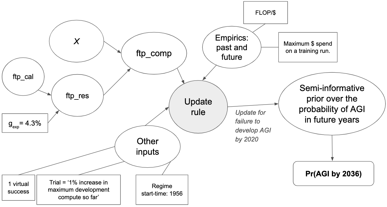
The tables below show how the output of this methodology depends on ftp_cal, X, and your estimate of the largest training run that will have occurred by 2036.90 (I’ve highlighted the inputs and output for my central estimate in bold.)

CONSERVATIVE: $100 MILLION SPEND BY 2036		PR(AGI BY 2036)
		CALENDAR YEAR TRIAL DEFINITION	COMPUTE TRIAL DEFINITION
			X = 1	X = 5	X = 10
ftpcal	1/50	12%	16%	14%	11%
	1/100	8.9%	15%	11%	8.7%
	1/300	4.2%	13%	7.0%	4.4%
	1/1000	1.5%	8.6%	3.0%	1.6%
	1/3000	0.52%	4.4%	1.1%	0.58%

AGGRESSIVE: $100 MILLION SPEND BY 2036		PR(AGI BY 2036)
		CALENDAR YEAR TRIAL DEFINITION	COMPUTE TRIAL DEFINITION
			X = 1	X = 5	X = 10
ftpcal	1/50	12%	26%	23%	20%
	1/100	8.9%	25%	20%	15%
	1/300	4.2%	22%	13%	8.1%
	1/1000	1.5%	15%	5.5%	3.1%
	1/3000	0.52%	8.1%	2.1%	1.1%

With this methodology, even extreme initial skepticism (ftp_cal ~ 1/3000) can potentially be overcome by the fast increase in C.91

Based on the above tables, my central estimate increases to ~10%92 and my range increases to 2 – 25%.93 Considering the biological hypotheses below will raise this central estimate to 15%, mostly via putting 50% weight on a late regime start-time, but leave the range intact.

6.2.2.2 Use biological hypotheses to estimate the median compute for developing AGI

This method of estimating ftp_comp involves speculative claims about the computational power needed to replicate the brain’s performance on cognitive tasks (‘brain compute’), the computation needed to redo the process of evolution (‘evolutionary compute’), and the relevance of these quantities to creating AGI. Thus, it departs somewhat from the spirit of the report. However, I found that the conclusions were broadly similar to conclusions I got using other methods, so I thought I would include them anyway because they seem to increase the robustness of the findings.

In particular, I consider three biological hypotheses you might have for the computation needed to develop AGI: the lifetime learning hypothesis, the evolutionary hypothesis, and the brain debugging hypothesis. Though the hypotheses are highly speculative, they may collectively provide some guide as to the amount of computation that might be needed to develop AGI, and so it may be useful to incorporate them into our framework.

Lifetime learning hypothesis. As a child grows up to be an adult, it learns and becomes generally intelligent. Central to this learning process is the computation happening in the child’s brain. Call the amount of computation that happens in a child’s brain until they’re 30 years old ‘lifetime compute’. Perhaps AI R&D will be able to produce a generally intelligent system with less computation than this, or perhaps it will take more. Overall there’s a 50% chance we’ll have developed AGI by the time C equals lifetime compute.

Evolutionary hypothesis. Evolution has selected for generally intelligent systems – humans. The important computation for this process was the computation that happened inside the nervous systems of animals throughout evolution. Call this amount of compute ‘evolution compute’. Perhaps AI R&D will be able to develop a generally intelligent system with less computation than evolution, or perhaps it will take more. Overall there’s a 50% chance we’ll have developed AGI by the time C equals evolution compute.94

Brain debugging hypothesis. The first AGI we develop will probably use as much or more computational power than the human brain. Further, we’ll need to run the AGI for at least two weeks while we develop it, to iron out any bugs and check that it works. Call the compute required to run the human brain for two weeks ‘brain debugging compute’. So there is a 0% chance we will develop AGI before the point at which C equals brain debugging compute. (This means the regime start-time cannot be before this point.)

To actually use these hypotheses, we need estimates of the compute quantities they involve:

• My colleague Joe Carlsmith has written a report on how much computational power might be needed to match the human brain (see blog). His median estimate is that it would take FLOP/s to match the brain’s cognitive task performance.
  • This implies that lifetime compute is 10¹⁵ × 10⁹ = 10²⁴ FLOP (there are ~10⁹ seconds in 30 years).
  • It also implies that brain debugging compute is 10¹⁵ × 10⁶ = 10²¹ FLOP (there are ~ 10⁶ seconds in two weeks).
• My colleague Ajeya Cotra estimates that evolution compute is 10⁴¹ FLOP in her draft report.

Though I don’t literally believe any of the biological hypotheses and am not confident in the exact numerical estimates above, I believe they are useful anchors for our views about ftp_comp and pr(AGI by 2036).

How can we incorporate these biological hypotheses into the semi-informative priors framework? The the brain debugging hypothesis can be used to specify a (very recent) regime start-time,95 and then the lifetime learning and evolutionary hypotheses can be used to calculate ftp_comp,96 I consider a two methods of incorporating the hypotheses into the framework:

• Evolutionary anchor: Use the brain debugging hypothesis to choose the regime start-time and the combine the evolutionary and brain debugging hypotheses to choose the first-trial probability. Ignore the lifetime learning hypothesis.
• Lifetime anchor: Use the lifetime learning hypothesis to choose the first-trial probability and leave the regime start-time at 1956 as in the previous section.97 Ignore the evolutionary and brain debugging hypotheses.98

The following table shows pr(AGI by 2036) for both these uses of bio-anchors, along with my central estimates from the previous section.

INCREASE IN COMPUTE SPEND	HOW ARE BIOLOGICAL HYPOTHESES INCORPORATED?		RESULTS OF PREVIOUS SECTION: FTPCAL = 1/300, X = 5
	LIFETIME ANCHOR	EVOLUTIONARY ANCHOR
Conservative: $100 million spend by 2036	8.9%	13%	7%
Aggressive: $100 billion spend by 2036	16%	22%	13%
Equal weight on conservative and aggressive spend	12%	17%	11%

A few things are worth noting:

• The probabilities are higher for evolutionary anchor than for lifetime anchor. This is somewhat surprising, as the evolutionary anchor has a smaller first-trial probability than lifetime anchor.
  • The explanation is that the evolutionary anchor has a late regime start-time – when C equals brain debugging compute – so doesn’t update much on the failure to create AGI by 2020. Meanwhile the lifetime anchor has an earlier regime start-time and assigned 50% to success by 2020, so updates significantly based on the failure to create AGI by 2020.
• The bottom line probabilities are slightly higher than the compute-based results from the previous section. For the lifetime anchor this is driven by a higher first-trial probability. For the evolutionary anchor, the bigger contributor is the late regime start-time.
• The biological hypotheses suggest a value for ftp_comp in the higher end of the range suggested by the previous section.99 The values for ftp_comp implied by evolutionary anchor and lifetime anchor are ~1.5X higher than my central value from the previous section (ftp_cal = 1/300 and X = 5).100

6.2.2.2.1 Log-uniform distributions over compute

I want to flag an interesting alternative approach to incorporating biological hypotheses into a simple priors model. This approach thinks that AGI is unlikely to be developed before brain debugging compute but is very likely to be developed by evolution compute. Its unconditional distribution over “How much compute is needed to develop AGI?” is log-uniform between brain debugging and evolution compute.

Note that evolutionary anchor is importantly different to the log-uniform model. The difference is most clearly shown by the diagrams below. In evolutionary anchor, the unconditional probability of success is skewed towards earlier trials (towards brain debugging compute and away from evolutionary compute) because i) later trials won’t happen if earlier trials succeed and ii) our confidence that the next trial will succeed even if it happens decreases over time. On the log-uniform model, by contrast, later trials have equal unconditional probability to earlier trials. This means that on the log-uniform model the conditional probability of success given that the previous trials have failed – E(p) in our model – actually increases for later trials.

The log-uniform compute model, with 20% probability set aside for greater than evolution compute, outputs pr(AGI by 2036) of 15% for conservative spend estimates, or 29% for aggressive ones.101 This is higher than the other models considered so far. I believe that the log-uniform model is more appropriate than the semi-informative priors framework if you think we’re very likely to have developed AGI by the time we reach evolution compute, as the framework is not well suited for modeling ‘end-points’ like this.102

6.2.2.2.2 Plots of distribution from biological hypotheses

I’ve plotted the conditional and unconditional probabilities that these three biological hypothesis based models assign to creating AGI at various levels of development FLOP. 103

 

 

 

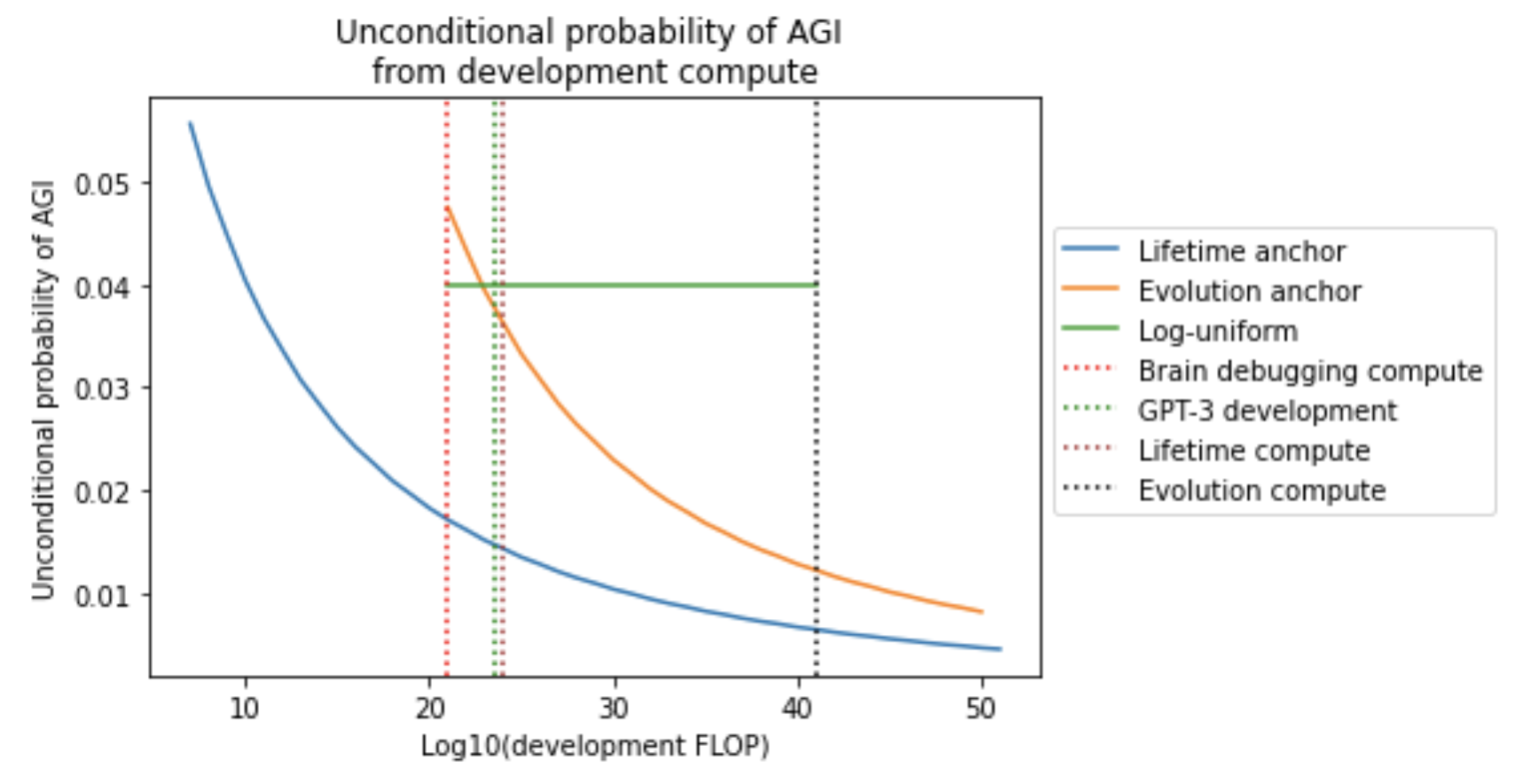
6.2.3 All things considered bottom line with the compute trial definition

To incorporate fast-increasing use of compute to develop AGI systems into the semi-informative priors framework, we need some way of estimating ftp_comp. I’ve considered two methods. The first derives ftp_comp from ftp_res – which was itself derived from ftp_cal – and an assumption about the relative importance of researcher-years and compute. The second derives ftp_comp from biological hypotheses about the median compute required for AGI. I also put weight on using a log-uniform distribution, which gives results consistent with the upper-end of this range.

The following table shows the central estimates of pr(AGI by 2036) of all the models considered in this section. (For the penultimate column, I also include the range of plausible values from the table.)

INCREASE IN COMPUTE SPEND	BIOLOGICAL HYPOTHESIS			SPECIFY RELATIVE IMPORTANCE OF RESEARCH AND COMPUTE FTPCAL = 1/300, X = 5	WEIGHTED AVERAGE
	LIFETIME ANCHOR	EVOLUTIONARY ANCHOR	LOG-UNIFORM
Conservative: $100 million spend by 2036	8.9%	13%	15%	7.0% (1.5 – 15%)	11%
Aggressive: $100 billion spend by 2036	16%	22%	29%	13% (3 – 25%)	20%
Equal weight on conservative and aggressive spend	12%	18%	22%	11%	15%

The biological hypotheses give results towards the upper end of the range in the previous section because they have slightly higher first-trial probabilities. The evolutionary anchor and log-uniform give especially high probabilities as they have late regime start-times. I am happy to simply weigh the four views in the table equally (as shown in the last column), which corresponds to placing 50% weight on a late regime start-time in the context of compute-based trials.104

I place equal weight on conservative and aggressive spend, so for compute trials my overall central estimate is 15% and my preferred range is 2 – 25%.

6.3 Varying the number of virtual successes and the regime start-time

When the trial definition was ‘a calendar year’ I found that varying the regime start-time and number of virtual successes inputs didn’t affect the bottom line by much. This story is more complicated when we define trials in terms of researcher-years and compute. The basic reason is that these trial definitions are more surprised by the failure to develop AGI by 2020, and so the update from this failure is bigger. The regime start-time and number of virtual successes affect the size of this update, so can significantly impact the bottom line.

In brief:

• Fewer virtual successes amplifies the size of the update from failure. This curbs the high-end values for pr(AGI by 2036), typically bringing them down to below 10%.
• Late regime start-times mostly eliminate the update from the failure so far. This significantly boosts high-end values of pr(AGI by 2036), potentially up to 25%.
• If you use fewer virtual successes and a late regime start-time, the high-end pr(AGI by 2036) is boosted.
  • The effects of these two changes point in opposite directions, but the late regime start-time wins out.
• Very early regime start-times still make little difference to the analysis.

Personally, I find that the effects of late regime start-times and fewer virtual successes are mostly a wash on my overall bottom line.

The rest of this section explains the effects of these two parameters in more detail, but you may be happy to move on to the next section.

6.3.1 Number of virtual successes

Throughout Section 6 we’ve assumed 1 virtual success. My preferred range for the number of virtual successes is 0.5 – 1, and so this section summarizes how the bottom line differs if I used 0.5 instead of 1.

I reran this section’s analyses with 0.5 virtual successes.105 The table summarizes the changes to my preferred range and central estimate. In this analysis, I placed no weight on models with late regime start-times (except for in brackets, where I show the results when 50% weight is placed on late regime start-times106).

PR(AGI BY 2036)
	1 VIRTUAL SUCCESS	0.5 VIRTUAL SUCCESSES
Researcher-year – low	2.3%	2.1%
Researcher-year – central	7.9%	5.8%
Researcher-year – high	15%	8.8%
Compute – low	1.6%	1.5%
Compute – central107	12% (15%)	9.2% (14%)
Compute – high108	22% (25%)	13% (22%)

The low-end estimates aren’t affected much. The central and high-end estimates are reduced quite significantly. They tend to be pushed down below 10%, and often move half of the way towards 4% – e.g. from 15% to 9%. (When 50% weight is put on late regime start-times, as for the numbers in brackets, the effect is smaller.)

The table probably overestimates the impact of using 0.5 virtual successes rather than 1. As discussed earlier, if we reduce the number of virtual successes, we should increase the first-trial probability somewhat to compensate.

Overall, reducing the number of virtual successes makes more difference than when a trial was a ‘calendar year’, pushing probabilities down below 10% and towards 4%, but has little effect on probabilities below 5%. This effect can be dampened by putting weight on late regime start-times.

6.3.2 Regime start-time

With trials as calendar years, I argued that considering late regime start-times will slightly increase your top-end probabilities considering early regime start-times will push your probability down towards the lower end of your preferred range.

Late regime start-times

The effects of late regime start-times are more significant for the compute and researcher-year trial definitions. The late start-time of evolutionary anchor raises its pr(AGI by 2036) from ~12% to ~17%.109 A similar story is true of the researcher-year trial definition: a late regime start-time of 2000 would increase my central estimate from 8% to 10% and my high-end from 15% to 25%.110

The reason is that the update from failure to create AGI between 1956 and 2020 is significant for these trial definitions; this update is mostly eliminated when the regime start-time is 2000.

Very early regime start-times

Early regime start-times seem less plausible for these two trial definitions as before 1940 there were no AI researchers and no digital computers. In any case, I believe we can simply re-run the earlier argument in Section 5.3 that their potential effect is limited. In brief, even if we use a very early regime start-time, the update from failed trials will only be moderate because very few trials occur each year before 1940.

6.3.3 Summary – my preferred ranges before and after varying the other inputs

This summarizes what my preferred ranges for pr(AGI by 2036) before this section, assuming 1 virtual success and a regime start-time of 1956 (except for the late start-times considered in the compute analysis).

	PR(AGI BY 2036)
TRIAL DEFINITION	LOW-END	CENTRAL ESTIMATE	HIGH-END
Calendar year	1.5%	4%	9%
Researcher-year	2%	8%	15%
Compute111	2%	15%	25%

Having considered other values for the regime start-time and the number of virtual successes, here’s are my ranges:112

	PR(AGI BY 2036)
TRIAL DEFINITION	LOW-END	CENTRAL ESTIMATE	HIGH-END
Calendar year	1%	4%	10%
Researcher-year	2%	8%113	15%114
Compute115	2%	13%	22%

Overall there is little change to my bottom line because I take late regime start-times and 0.5 virtual successes somewhat seriously, and their effects on my bottom line roughly balance out.116 If the reader takes one of these possibilities more seriously than the other, their bottom line may shift significantly. If you fully embrace both possibilities, your bottom line will increase as fewer virtual successes won’t undo the effect of a late regime start-time.

6.4 Summary – other trials definitions

As the above tables indicate, the analysis suggests that defining trials in terms of researcher-years or compute can significantly increase your bottom line. My central estimate moves from 4% to 8% with researcher-year trial definitions, and then to 15% with compute trial definitions. My high-end increases even more from 10% to 15% (researcher-year) and then to 22% (compute). My low-end is not significantly affected.

How should we form an all-things-considered view given these different trial definitions? I propose taking a weighted average.117 There are several factors which might affect the weight you give to each definition.

• You should give trial definitions less weight to the extent you think they involve speculative reasoning.
• You might want to give more weight to the ‘researcher year’ and ‘compute’ trial definitions, as they condition on more information about the inputs to AI R&D.
• You should give more weight to ‘calendar year’ definitions if your ftp_cal already priced in the empirical considerations discussed when considering the other definitions. In particular, the larger pr(AGI by 2036) for the ‘researcher-year’ and ‘compute’ definitions are driven by the fast increase of the number of researchers and the compute used in AI R&D. You might have chosen ftp_cal with the expectation that these R&D inputs would grow quickly, or implicitly anchored off other R&D efforts where research effort grew unusually quickly. I tried to avoid doing this, so for me this factor is not significant.

Overall, I find the first two factors to be roughly equally persuasive and I assign ⅓ weight to each of the trial definitions that I’ve considered. Taking a weighted average of the low-end, central estimate and high-end individually produces the following result: a range of 1.5% – 16% and a central estimate of 8%.

7 Model extensions

This section analyzes three extensions to the semi-informative priors model.

Here’s a brief summary of the extensions and their effects on the bottom line:

1. Model AGI as conjunctive (here):
   • Description. In this model, to develop AGI we must complete multiple independent tasks. When calculating pr(AGI by 2036 | no AGI by 2020) I don’t remain agnostic about how many conjuncts are completed in 2020, only assuming that ≥1 conjunct(s) are incomplete.
   • Results. The conjunctive model seems like a slightly more realistic version of the non-conjunctive model we’ve used throughout this report. Believing that AGI is conjunctive might make you lower your pr(AGI in first 100 years) somewhat. However, if we hold pr(AGI in 100 years) fixed, a conjunctive model has a slightly larger pr(AGI by 2036) than a non-conjunctive model. This is because conjunctive models dampen the probability of success in the early years of effort, and so the (fixed) probability of success is concentrated in later years instead.
2. Updating a hyper prior (here):
   • Description. Assign weights to the different update rules considered in this document and update these weights based on the failure to create AGI so far. Rules are down-weighted to the extent that they expected AGI would already be developed by 2020.
   • Results: This tends to push the bottom line down towards the 5 – 10% range but not below it. It significantly down-weights the most aggressive ‘researcher-year’ and ‘compute’ update rules. But when update rules have a late regime start-time, hyper prior updates make little difference; in this case the bottom line can remain above the 5 – 10% range.
3. Assign some probability that AGI is impossible (here):
   • Description. Place some initial weight on AGI being impossible, and update this weight based on the failure to develop AGI by 2020. This is a special application of a hyper prior.
   • Results. Assigning 20% to this possibility tends to push your overall bottom line down into the range 3 – 10%, but not below. However, update rules with late regime start-times are slightly less affected – such rules can still drive an overall pr(AGI by 2036) above 10%.

7.1 Model AGI as conjunctive

In this section I:

• Explain the motivation for modeling AGI as conjunctive (here).
• Describe the conjunctive model (here).
• Discuss implications of the conjunctive model (here).
• Clarify the model’s assumptions (here).
• Summarize the key takeaways (here).

7.1.1 Why model AGI as conjunctive?

Suppose you were modeling the prior probability that we’ll develop a unified theory of physics AND put a person on Mars AND make a building >1km tall by 2036. It would be natural to model the chance of success for each conjunct separately and multiply together the three results. This is because each conjunct is fairly independent of the others, and the initial claim divides very naturally into three conjuncts.

One might think that AGI is similarly conjunctive. Here are a brief argument for thinking so:

1. Many ways of defining AGI are inherently conjunctive. AGI requires high capabilities in multiple domains, and the claims about separate domains are conjunctive. Some example definitions that follow this pattern:
   • Mass automation definition: AGI = automating driving and automating teaching and automating consulting and…
   • Subdomains of AI R&D definition: AGI = human level vision and natural language processing and planning and social skills and…
   • Pre-requisites definition: AGI = good exploration and good hierarchical planning and good memory and sample efficient learning and…
   • Cognitive tasks definition: AGI = human abilities in virtually all cognitive domains.
2. A non-conjunctive model is only accurate if all these conjuncts are highly correlated with each other. If any two conjuncts are independent of each other, a conjunctive model is better.
3. So we should assign some weight to the possibility that AGI is a conjunction of (a smaller number of) independent conjuncts.

This argument suggests we think about the conjuncts as different capabilities. But we could also think of them as different breakthroughs that may be required to develop AGI.

7.1.2 How the conjunctive model works

In the model, developing AGI requires achieving multiple independent conjuncts. Each conjunct is modeled exactly as I’ve previously modeled AGI as a whole. For simplicity, each conjunct has the same inputs (first-trial probability, regime start-time, etc.).

So if there are four conjuncts, I’d calculate the probability of developing AGI in the first N years of effort as follows:

1. Choose a conjunct, and calculate the probability of achieving it in the first N years of effort.
   • This calculation uses the semi-informative framework I explained in Section 3. We have a prior E(p) that the first year will succeed, update E(p) downwards to calculate the conditional probability that the second year succeeds if the first year fails, and combine the conditional probabilities for the first N years.
2. The probabilities of the other three conjuncts succeeding the the first N years are all the same as they have the same inputs.
3. Multiply together the four probabilities.
4. We can do this because we assume the conjuncts are independent: knowing that we’ve achieved one conjunct doesn’t affect our probability of achieving any of the others.

As always, to calculate pr(AGI by 2036) we must condition on the failure to succeed by 2020. When doing this, we only condition on the minimal claim that “at least one conjunct is not yet achieved”. We don’t condition on the stronger claim “none of the conjuncts have been achieved” or make an assumption about the proportion of conjuncts that have been achieved.118

In the analysis below, I use the following inputs:

• Trial definition: calendar year
• Regime start-time: 1956
• Number of virtual successes: 1

7.1.3 Implications of the conjunctive model

7.1.3.1 Dampen probability of success near the start

In the original non-conjunctive model, the conditional probability of achieving AGI, E(p), is highest in the first trial and falls off over time. In the conjunctive model, however, this probability starts very low, increases significantly, and then starts to slowly fall off.

 

 

The blue line is simply the non-conjunctive model we’ve used throughout the report. The orange and green lines add progressively more conjuncts. The first-trial probabilities for the three models were chosen so that the probability of developing AGI in the first 100 years is ~25%. The graph shows that conditional probability of the conjunctive models overtake the non-conjunctive model after 25 – 50 years.119

This corresponds to the following cumulative probabilities of developing AGI:

 

 

I find the behavior of the conjunctive model intuitive – it seems like AGI had a larger chance of being created in 1970 than 1957.

7.1.3.2 We can convert non-conjunctive models into conjunctive models to make them more realistic

Non-conjunctive models unrealistically imply that AGI was more likely to be developed in the first year of effort than in any other. We can use the conjunctive model to estimate how we might adjust for this problem.

My proposal for doing this is as follows:

1. Adjust the first-trial probability of your preferred non-conjunctive model to account for the possibility that AGI consists of multiple conjuncts.
   • I personally already took this consideration into account in Section 4. The examples of historical technological R&D that I used to inform my first-trial probability (e.g. here and here) are plausibly conjunctive, just like AGI is. I think AGI is particularly conjunctive, and use this to motivate the small first-trial probability of 1/300 here.
   • If you feel that AGI is unusually conjunctive, and you hadn’t previously priced this into your first-trial probability, you should adjust your first-trial probability accordingly.
2. Calculate the cumulative probability of developing AGI in the first N years, according to this adjusted non-conjunctive model.
3. Choose N so that you feel comfortable with the model’s predictions over that time horizon.
4. For example, I considered N = 50 and N = 100 when choosing my first-trial probability in Section 4, so I would use one of these values.
5. Take a conjunctive model with the same inputs as your non-conjunctive model, except for the first-trial probability.
6. You could choose a particular number of conjuncts you find roughly plausible, or try a range of possibilities as I do below.
7. Choose the first-trial probability of the conjunctive model so the cumulative probability of developing AGI in the first N years is the same as the non-conjunctive model.
8. This assumption allows us to study the effect of more conjuncts on the shape of the distribution, as distinct from the fact that if AGI is more conjunctive then we should assign less probability to it being developed in a particular time frame. The latter point was accounted for in Step 1.
9. Look at how pr(AGI by 2036) differs in your conjunctive model. The difference is an estimate of the adjustment you should make to the predictions of the non-conjunctive model.

What does this methodology imply for pr(AGI by 2036)? To get a rough answer for this question, I compared the probabilities of the non-conjunctive and conjunctive models, holding pr(AGI in the first 100 years) fixed between them. I looked at the conditional probabilities, defined as pr(AGI by year Y | no AGI by year Y – 1). [In the non-conjunctive model, these probabilities are simply equal to E(p).]

 

 

After 35 years, the models differ by less than a factor of 2. The conjunctive models have a slightly higher pr(AGI by 2036).

	PR(AGI BY 2036)
FIRST-TRIAL PROBABILITY FOR 1 CONJUNCT	1 CONJUNCT	2 CONJUNCTS	100 CONJUNCTS
1/50	12%	14%	15%
1/300	4.2%	5.4%	6.9%
1/1000	1.5%	2.1%	2.9%
1/3000	0.5%	0.8%	0.7%

The intuitive reason for the upwards adjustment is that I am holding pr(AGI in the first 100 year) fixed and the conjunctive model shifts probability from the earliest years of development to later years. Importantly, I am remaining agnostic about how many conjuncts have been completed, only updating on the fact that they haven’t all been completed. If I updated on the further claim that there are multiple conjuncts remaining, there might be a downwards adjustment.

You get the same qualitative result holding (e.g.) pr(AGI in the first 50 years) fixed, rather than pr(AGI in the first 100 years).120

If you instead hold pr(AGI in first 500 years) fixed, the probabilities are dampened for longer. If pr(AGI in first 500 years) is sufficiently low then there can be a downwards adjustment to pr(AGI by 2036). This suggests one route to a very low bottom line: use first-trial prior = 1/1000, use a model with 100 conjuncts, hold fixed pr(AGI by the first 500 years). Essentially, this amounts to saying that AGI is so hard, and contains so many independent conjuncts, that there’s negligible probability that it will be developed with 100 years of effort. To me, it seems unreasonable to be confident in this position given the reference classes discussed in Section 4, but reasonable to assign it some weight.121

7.1.3.3 Generate low pr(AGI by 2036)

You could potentially use the conjunctive model to lower your pr(AGI by 2036) by additionally assuming that multiple independent conjuncts still have not been solved as of 2020. However, this involves making controversial assumptions about state of the art AI R&D that this project is meant to avoid, so I only discuss this application in an appendix.

7.1.4 Clarifying the model assumptions

Importantly, the model assumes that the conjuncts are independent of each other. Mathematically:

pr(Conjunct A is solved) = pr(Conjunct A is solved | Conjuncts B, C… Z are solved)

This independence assumption blocks an inference along the lines of “we solved conjuncts B and C really easily, so conjunct D is also likely to be easy”. The only information we have about the difficulty of conjunct D is the fact that we haven’t yet completed it; its difficulty is independent of the difficulty of the other conjuncts. This assumption is fairly unrealistic, but it only needs to hold approximately for two of the conjuncts that make up AGI. The power of the independence assumption is highlighted by an example I explain in the appendix here.

What the model does not assume:

• We know the specific conjuncts AGI decomposes into.
• Each conjunct is a stepping stone towards AGI.
• This is not a natural interpretation of the model, as the conjuncts don’t need to be completed sequentially.
• Rather, each conjunct should be thought of as the endpoint of a certain line of development (e.g. “automating teaching”) or as a breakthrough that’s necessary for AGI.

7.1.5 A sequential model

I’ve briefly investigated a sequential model, where multiple steps must be completed one after the other. Each step is modeled exactly as in the conjunctive model, with uncertainty about its difficulty. As before the steps are assumed to be independent: if one step is completed slowly or quickly, this isn’t correlated with the difficulty of the other steps. At most one step can be completed each trial (see code here).

I found the adjustments from this sequential model were the same as from the conjunctive model discussed above, but somewhat amplified. When we hold pr(AGI in 100 years) constant, the probability of success in early years is dampened for longer, and the probability of later years is boosted by more to compensate. When the model has 10 steps, the annual probability of developing AGI overtakes the non-conjunctive model after about 50 years of effort.

 

 

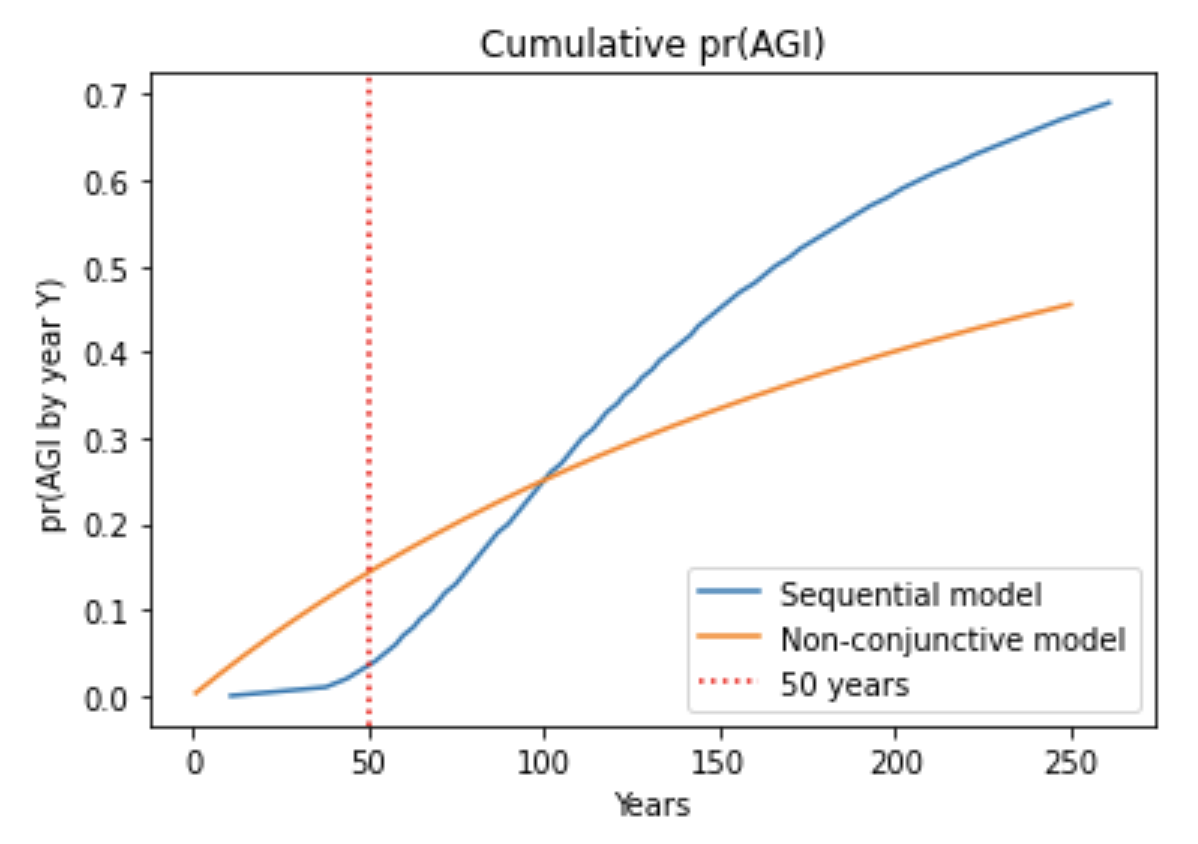
Increasing the number of necessary steps amplifies these effects even more: the probability stays low for longer and the probability of later years is boosted by more to compensate.122

The adjustment to pr(AGI by 2036 | no AGI by 2020) from using a sequential model depends on conditional probability of success: pr(AGI in year X | no AGI by year Y -1). The sequential model is not analytically tractable, but I ran simulations to calculate this quantity. After 50 years, both models agree about the conditional probability of success within a factor of ~2.

 

 

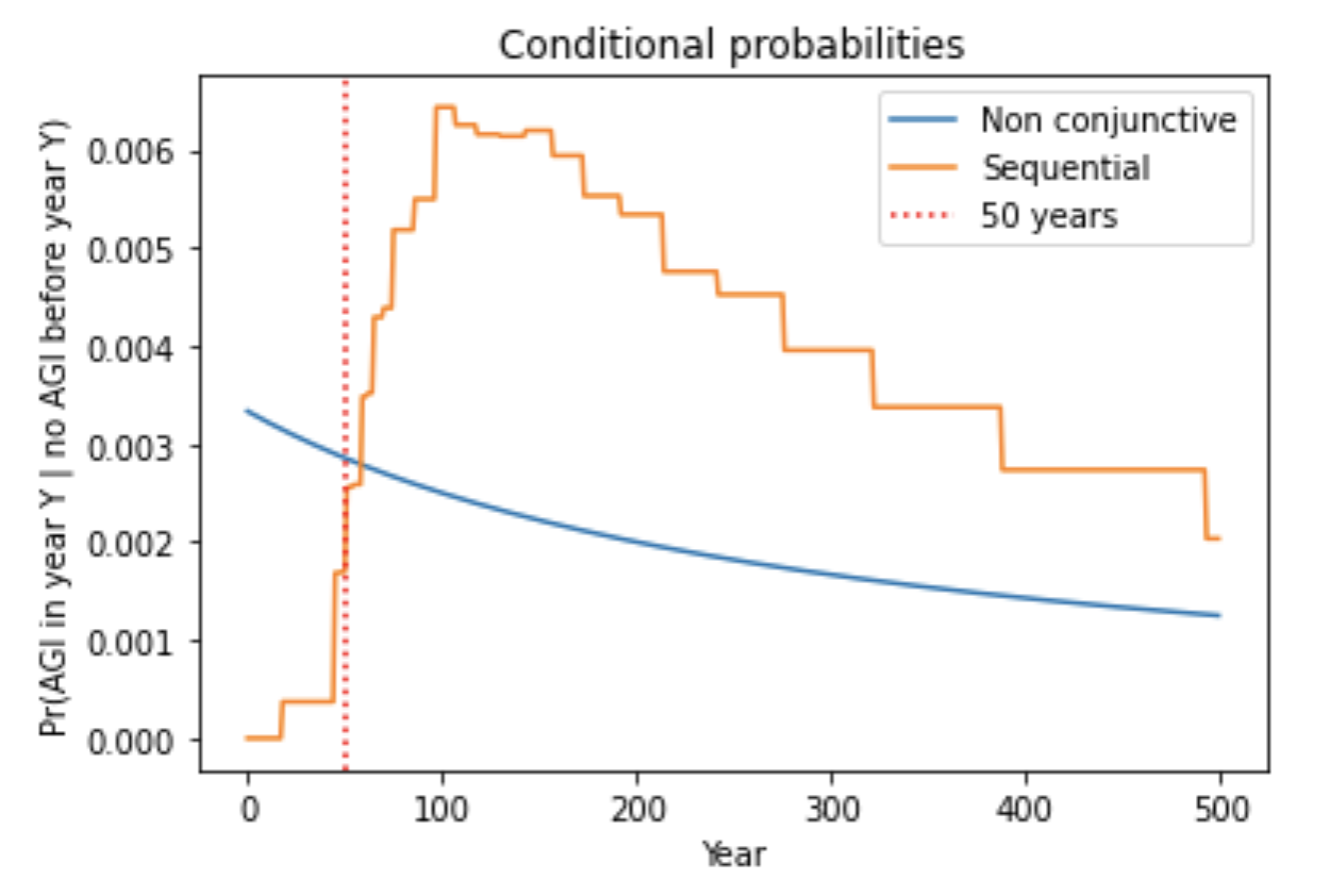
It’s worth emphasising that the reason the models give similar predictions is because the sequential model remains agnostic about how many sequential steps still remain. It is only updated on the binary fact AGI hasn’t been fully achieved. For all it knows, only one step remains! This is consistent with this report not taking into account evidence like “we’re x% of the way to completing AGI”, or “if we do steps XYZ, we’ll develop AGI”.

In addition, this result crucially assumes pr(AGI in the first 100 years) is held fixed between the two models. Again, the thought here is that our first-trial probability (in the non-conjunctive model) already prices in the belief that AGI requires a sequence of developments. If you want to lower pr(AGI in the first 100 years) when moving to a sequential model, you need to make that adjustment by hand.

7.1.6 Possible future work

Much more could be done to extend this basic framework. For example, we could consider disjunctive requirements in addition to conjunctive ones, or both at the same time. Perhaps most interesting would be to model uncertainty about the number of conjuncts.

7.1.7 Takeaways from the conjunctive model

The conjunctive model seems like a slightly more realistic version of the non-conjunctive model we’ve used previously, dampening the probability of success in early years. Using a sequential model gives similar qualitative results, but to a more extreme degree.

I suggested a method for adjusting the probabilities of non-conjunctive models to approximate that from a more realistic conjunctive model. The method implies that we should moderately increase pr(AGI by 2036), multiplying it by a factor of 1 – 2. Crucially, this model made no assumption about how many conjuncts we’ve completed as of 2020; this is why it makes similar predictions to the non-conjunctive model.

7.2 Updating a hyper prior

There are many inputs that determine our update rule, and many possible values for each input. It seems reasonable to be uncertain about what the correct inputs are. So we can take a weighted average across many different update rules. I assign weight to each rule in proportion to my confidence that it is correct.

In this case, we should update these weights based on how surprised each update rule is that AGI has not been developed by 2020. Rules that confidently expected AGI by 2020 will be down-weighted, update rules that were skeptical will be up-weighted.123 We then use the 2020 weights to calculate pr(AGI by year X).124

In other words, we should place a hyper prior over update rules and update this hyper prior for each year that we haven’t developed AGI.

The initial weight we assign to each rule should not take into account the failure to develop AGI by 2020. For example, we should not give a small initial weight to an update rule because it predicts a high probability of developing AGI early on.

 

 

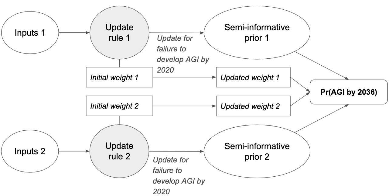
In this appendix I argue that we must use a hyper prior if we place weight on several different update rules – in fact I show that not doing so leads to inconsistent predictions. Ultimately, updating the weights of a hyper-prior is just another example of Bayesian updating, and the standard arguments for updating apply.

I investigated the consequences of using a hyper-prior for two inputs: the first-trial probability (here) and the trial definition (here). I chose these inputs because they drive significant uncertainty about the bottom line.

In brief, updating a hyper prior tends to push the bottom line down towards the 5 – 10% range but not below it. But if you have a late regime start-time, hyper prior updates make little difference even if your bottom line is >10%.

7.2.1 Effect of hyper prior updates: first-trial probability

Suppose you initially have equal weight on multiple different first-trial probabilities. What is the effect of hyper prior updates? The following table assumes that:

• Trial definition: calendar year
• Regime start-time: 1956
• Virtual successes: 1

FIRST-TRIAL PROBABILITIES ON WHICH YOU INITIALLY HAVE EQUAL WEIGHT	PR(AGI BY 2036) WITH STATIC WEIGHTS	PR(AGI BY 2036) WITH HYPER PRIOR UPDATES	WEIGHTS IN 2020125
1/100, 1/1000	5.2%	4.4%	39%, 61%
1/10, 1/100	13%	10%	17%, 83%
1/10, 1/100, 1/1000	9.5%	5.4%	7.4%, 36%, 56%
1/1000, 1/10,000	0.82%	0.80%	49%, 51%

For first-trial probabilities in my preferred range [1/1000, 1/100], hyper prior updates make <1% difference to the bottom line. For first-trial probabilities above this range, the difference is more significant, pushing pr(AGI by 2036) down into the 5 – 10% range.

This is consistent with the equivalent analysis for different trial definitions. This analysis also shows that hyper prior updates have very little effect when a late regime-start time is used.

7.2.2 Should this change our preferred number of virtual successes?

We earlier chose the range [0.5, 1] for the number of virtual successes based primarily on these values leading to reasonable updates from failure to develop AGI so far. When we update a hyper prior, we increase the size of the update from this failure. If we wish to keep the overall size of this update fixed, we should slightly increase the number of virtual successes when we use a hyper-prior. It turns out the size of the required increase is very small, around ~0.2.126

7.3 Allow some probability that AGI is impossible

AGI may turn out to be impossible.127 But the priors we’ve used so far all imply that – assuming we continue to increase the inputs to AI R&D without limit – AGI will happen eventually, even if it’s not for a very long time.

How would assigning some probability to AGI being impossible change the bottom line?

I found that the effect is to push your bottom line down into the 3 – 10% but not below, with a maximum reduction of about 5%. First I describe how I investigated this question (here), and then summarize the results (here).

7.3.1 Investigation

To model this, I put some initial weight on AGI being possible and some on it being impossible. Then we update these weights over time, increasing the weight ‘AGI impossible’ for each year that AGI isn’t developed. This is an application of the hyper prior updates discussed in the previous section.

I investigated how pr(AGI by 2036) changes when we assign 0% vs 20% initial weight to ‘AGI impossible’, with the rest of the weight on some other update rule. For the other update rule, I varied the first-trial probability and used the following inputs:

• Trial definition: calendar year
• Regime start-time: 1956
• Virtual successes: 1

FIRST-TRIAL PROBABILITY	INITIAL WEIGHT ON ‘AGI IS IMPOSSIBLE’
	0%	20%
	PR(AGI BY 2036)	PR(AGI BY 2036)	WEIGHT ON ‘AGI IS IMPOSSIBLE’ IN 2020
1/1000	1.5%	1.2%	21%
1/300	4.2%	3.2%	23%
1/200	5.7%	4.3%	25%
1/100	8.9%	6.3%	29%
1/50	12%	7.9%	37%
1/20	16%	7.7%	52%
1/10	18%	5.9%128	67%

Overall, the effect is to push the bottom line down towards into the 3 – 10% range no matter how large your first-trial probability, but not reduce much below this range.129 The update towards AGI being impossible is fairly small for first-trial probabilities in the range [1/1000, 1/100]. This update would be much smaller for late regime start-times. (And of course, the update would be smaller if we assigned <20% initial weight to ‘AGI impossible’.)

I found broadly similar effects for other trial definitions (see results in this appendix), with slightly larger updates towards AGI being impossible because these trial definitions are more surprised by the failure to develop AGI so far.130

One interesting result from the final column of the table is that high values for the first-trial probability cause implausibly large updates towards ‘AGI impossible’ based on the failure to develop it so far. I see this as a strong reason to prefer first-trial probabilities below 1/20, and a weak reason to prefer values below 1/100.

7.3.2 Summary

If you assign 20% weight to AGI being impossible, and don’t increase your first-trial probability to compensate, this pushes your bottom line down towards the 3 – 10% range. Having updated on the failure to develop AGI by 2020, your weight on AGI being impossible will be in the 20 – 30% range.

The next section concludes.

8 Conclusion

This report aims to address the following question:

Suppose you had gone into isolation in 1956 and only received annual updates about the inputs to AI R&D (e.g. # of researcher-years, amount of compute131 used in AI R&D) and the binary fact that we have not yet built AGI? What would be a reasonable pr(AGI by year X) for you to have in 2021?

I articulated a framework in which specifying four inputs, and potentially some empirical data, defines an update rule. After updating on the failure to develop AGI by 2020, the update rule provides an answer to the above question. In this conclusion I summarize how each input affects pr(AGI by 2036), and explain how I reach my all-things-considered judgment. Currently my central value for pr(AGI by 2036) is 8%.

8.1 How does each input affect the bottom line?

This report has highlighted four key factors that bear on AGI timelines.

The first-trial probability. Whatever trial definition you use, the first-trial probability is a critical input to the bottom line. For very low values of this input, it is directly proportional to pr(AGI by 2036), but even for high values it makes a significant difference.132 The methods I’ve used to estimate and constrain this input involve difficult and highly subjective judgment calls. This parameter is both important and highly uncertain.

The trial definition. Defining trials in terms of researcher-years roughly doubled my bottom line compared to the calendar year baseline of 4%. Using compute-based trials more than triples my bottom line relative to this baseline. Deciding which trial definition to use, or how much weight to place on each, has a significant effect on pr(AGI by 2036).

Late regime start-times. If you have a high first-trial probability then the update from failure so far significantly reduces pr(AGI by 2036). This update can be mostly avoided if you also have a late regime start-time. So combining a high first-trial probability with a late regime start-time can leave you with a very large pr(AGI by 2036).133

Empirical forecasts. For the researcher-year and compute trial definitions, pr(AGI by 2036) depends on how much these inputs will increase by 2036.

The following table summarizes the effect of these inputs on pr(AGI by 2036):

TRIAL DEFINITION	LOW FTP, CONSERVATIVE FORECASTS134	CENTRAL FTP, CENTRAL FORECASTS	HIGH FTP, AGGRESSIVE FORECASTS	HIGH FTP, AGGRESSIVE FORECASTS AND LATE START-TIME (2000)
Calendar year	1.5%	4%	9%	12%
Researcher-year	2%	8%	15%	25%
Compute135	2%	15%	22%	28%

In addition, I’ve studied the effect of a few other factors.

Virtual successes. The numbers in the above table assume there’s 1 virtual success. Using 0.5 virtual successes instead pushes the bottom line down towards 4%, but not below this. For example, the numbers in the third column would be replaced by 6.5%, 9%, 13%. A late regime start-time dampens this effect, and so the 4th column would not be significantly altered.

Very early regime start-times. These have surprisingly little effect as it is reasonable to significantly down-weight years that occur long before 1956. I argued that this consideration at most suggests avoiding the top of my preferred range. This suggests that the update from failure to develop AGI by 2020 cannot justify pr(AGI by 2036) lower than ~1%, even when very early regime start-times are countenanced.

Modeling AGI as conjunctive. For me, this involved only a minor adjustment. I had already priced the possibility that AGI is conjunctive into my estimate of the first-trial probability, and so moving to a conjunctive model slightly increased my pr(AGI by 2036) slightly. This is because a conjunctive model moves probability mass from the early years of effort to later years, compared to a non-conjunctive model. The small adjustment might seem surprising – it’s because the conjunctive and sequential models make no assumption about the number of conjuncts that have been completed as of 2020.

8.2 Reaching an all-things-considered judgment

I believe the correct approach to forming an all-things-considered judgment is to place weight on multiple different update rules.136 In particular, we should place an initial weight on each update rule in accordance with its prior plausibility, then update these weights based on the failure to develop AGI by 2020. In this weighted sum, I think some weight (~10%) should be given to AGI being impossible.

I have used this process to construct a conservative, aggressive and central estimate of pr(AGI by 2036). I consider the conservative and aggressive estimates to be quite extreme as they are conservative / aggressive about multiple independent inputs.

My conservative estimate is 1%. This corresponds to a low first-trial probability, significant weight on calendar year trials and no weight on compute trials, no weight on late regime start-times, conservative empirical forecasts, and assigning 20% probability to AGI being impossible.137

My aggressive estimate is 18%. This corresponds to a high first-trial probability, significant weight on researcher-year and compute trials, significant weight on late regime start-times, aggressive empirical forecasts, and 10% probability on AGI being impossible.138

My central estimate is 8%. This corresponds to a central first-trial probability, equal initial weight on calendar year, researcher-year and compute trials, a small weight on late regime start-times, empirical forecasts near the middle of the range that I recommend, and 10% probability on AGI being impossible.139

	LOW-END	CENTRAL	HIGH-END
First-trial probability (trial = 1 calendar year)	1/1000	1/300	1/100
Regime start-time	Early (1956)	85% on early, 15% on late140	20% on early, 80% on late141
Initial weight on calendar-year trials	50%	30%	10%
Initial weight on researcher-year trials	30%	30%	40%
Initial weight on compute trials	0%	30%	40%
Weight on AGI being impossible	20%	10%	10%
g, growth of researcher-years	7.0%	11%	16%
Maximum compute spend, 2036	N/A	$1 billion	$100 billion
pr(AGI by 2036)	1.3%	7.5%	18%
pr(AGI by 2100)142	5.3%	20%	35%

It goes without saying that these numbers depend on many highly subjective judgment calls. Nonetheless, I do believe that the low-end and high-end represent reasonable bounds. I strongly encourage readers to take a few minutes to enter their own preferred inputs and initial weights in this tool, which also shows the assumptions for the low, high, and central estimates in more detail.

8.3 An important caveat

Perhaps we can rule out AGI happening in the next 5 years based on state of the art AI R&D.

Nothing in this report so far accounts for this possibility, because it is outside the purview of this project.

If you want to extend the framework to take this extra ‘information’ into account, the simplest strategy is to condition the model on the binary fact that AGI has not occurred by 2025 (rather than just by 2020 as I’ve done throughout). Those who think the evidence rules out AGI further into the future can use a later year than 2025, which is allowed in the tool.

When I additionally condition on the failure to develop AGI by 2025, my central estimate of pr(AGI by 2036) falls from 8.0% to 4.6%.

8.4 More general takeaways

Though this report focuses on pr(AGI by 2036), I believe there are some lessons from it that are more generally applicable. In particular:

• Skepticism about “we’ve been trying for ages and failing, so AGI is very unlikely to happen soon”. The update from failure to develop AGI to date doesn’t justify very low values of pr(AGI by 2036); at most it implies pr(AGI by 2036) < 5%.
  • The conservative values for pr(AGI by 2036) of ~1% are not driven by the update from failure so far. They are driven primarily by low values for the first-trial probability – 1/1000, for calendar year trials. The update from failure so far makes very little difference to this skeptical prior.
  • The significance from the failure so far is in curbing confidence in very short timelines. A regime start-time of 1956 tends to bring pr(AGI by 2036) down below 15% (see 3rd column in above table), or below 10% if we have 0.5 virtual successes. I argued that even extremely early regime-start times don’t bring pr(AGI by 2036) below 1%.
  • Even when considering very early regime start-times, that update from failure only implied pr(AGI by 2036) < 5%.
• Suspicion of ‘simple’ priors. Using a simple prior, like Laplace’s uniform prior over p, wasn’t a good way to generate reasonable probability distributions. This investigation updated me away from trusting priors (like Laplace’s) that appeal to simplicity, symmetry, entropy maximization, or other theoretical virtues. I believe you should try and ground your prior in some broader reference class wherever possible, perhaps placing weight in numerous different reference classes as I recommend.
• Suspicion of Laplace’s law. The following reasoning is suspect: ‘X has been going on for Y years so on average we should probably expect it to go on for about another Y years’. The reasoning is a result of applying Laplace’s rule of succession to predict the likely duration of X, with trials defined as increments of time. There are two problems with this reasoning, which both suggest the reasoning underestimates X’s future duration.
  • Firstly, we’ve seen that Laplace’s rule has an unreasonably large first-trial probability of 0.5. In this context, this corresponds to having 50% probability on Xfinishing in the first trial. But typically, even before Xbegins we have reason to expect it to last (on average) longer than a small increment of time. If so, Laplace’s rule will underestimate the future length of X. In the language of this report, we should use a smaller first-trial probability than Laplace when estimating the future length of X. For a vivid example, suppose someone said “How long will this new building last before it’s knocked down? I don’t know. It’s been standing for ~1 month so I’d guess it will stay standing for another month.” The problem with this reasoning is that we have other reasons, separate from its duration, to think it will last longer: most buildings last longer than 1 month. That said, the italicized reasoning may be approximately valid if Xhas already gone on for much longer than we expected – in this case the update from the duration dominates the effect of the first-trial probability and Laplace’s rule is approximately correct.
  • Secondly, if we used 0.5 virtual successes instead of 1 virtual success the italicized reasoning would become: ‘X has been going on for Y years so on average we should probably expect it to go on for about another 2Y years’. I think 0.5 virtual successes is plausible. This consideration again suggests that Laplace’s rule underestimates X’s duration.

9 Possible future research

9.1 Other way of estimating first-trial probability

Much more could be done to use empirical evidence to constrain the first-trial probability.

When a trial a calendar year:

• How often do STEM fields achieve their central aims? Get a list of ambitious goals that were as central to some STEM field as central AGI is central to AI R&D. How frequently are these goals achieved?
• How often do predictions of transformative technologies turn out to be correct? Gather a list (e.g. from 1850-1920) of predicted technological developments that, qualitatively speaking, seemed highly ambitious/crazy when predicted. What percentage of those predictions have come true?
• Perhaps by applying the methodology of this report to multiple different research goals, we could predict that the expected number of transformative developments that will occur is very high. How low should the first-trial probability be to avoid this? (See more here.)
• AGI would probably precipitate the automation of many jobs. Can we use the rate of automation to estimate AGI’s first-trial probability?

For researcher-year trial definitions.

• How much research effort did it take to achieve various other ambitious R&D goals (e.g. those discussed here)? Can we use this to estimate the first-trial probability for some researcher-year definitions?

Novel trial definitions:

• We might define a trial jointly in terms of both labour and compute inputs to R&D.
  • E.g. a trial is a 1% increase in A = L^αC^1-α.
  • How could we estimate the first-trial probability in this case?

9.2 Backtest methodology

I’d like to get a list of “things people in 1920 thought would be big deals in the 20th century” and see how this methodology would have fared. In particular, would it have been well calibrated?

9.3 Better data

My empirical forecasts, especially those for the growth of researcher-years, could be improved. This could significantly reduce uncertainty in the bottom line.

9.4 Explore sequential models

• Analyze more precisely the conditions under which the non-conjunctive framework makes similar predictions to sequential models.
• Consider disjunctive requirements, where there are many possible routes to AGI, in addition to conjunctive ones.
• Model uncertainty about the number of conjuncts.

10 Appendices

10.1 Under what circumstances does the semi-informative priors framework apply?

10.1.1 When is the model useful?

It is useful to distinguish between the circumstances under which the model applies, and those in which it is useful. Even if the model applies, it may not be useful if the evidence and arguments that it excludes are highly reliable and informative. In such a case, it may be more practical to try and find an all-things-considered view straight away rather than separately forming a semi-informative prior. For example, it would not be useful to form a semi-informative prior over the release date of the next iPhone if this date has already been announced.

One common reason the framework isn’t useful is that we can identify the ‘fraction of progress’ we have made towards a goal at any point in time. By comparing this metric at different times we can calculate our ‘rate of progress’ towards the goal, and extrapolate to calculate how long we have left until we achieve the goal. A good example of when this ‘rate of progress’ methodology is appropriate is for forecasting when the number of transistors in a dense integrated circuit (IC) might exceed a certain threshold, as under Moore’s law this quantity has risen at a fairly steady rate. Similarly, the ‘rate of progress’ methodology is commonly used for extrapolating US GDP per capita, which has risen steadily over the past 150 years.

Another common reason the framework might be less useful is if there are clear precursors to a project’s completion that we can identify in advance. For example, there would presumably be clear warning signs long in advance if we were to create a large civilization on Mars. In this case, the framework might still be useful for predicting when such clear signs may become apparent (see Fallenstein and Mennen (p.1) for more on this idea).

10.1.2 When is the model applicable?

Whether or not the model is useful, I believe the semi-informative priors framework is in principle applicable for forecasting the duration of a project when the evidence admissible to the report does not suggest a specific duration or a maximum duration, and when we are deeply uncertain about the difficulty of the project. Similarly, the framework is appropriate for forecasting events when the admissible evidence does not suggest a specific occurrence date or a latest possible occurrence date, and when we’re deeply uncertain about the annual likelihood of the event.

These conditions can hold for scientific R&D projects pushing the frontiers of knowledge, as it is likely that i) there are no closely analogous projects we can use to gain information about the project’s probable or maximum duration, and ii) we are deeply uncertain about how much progress is needed to reach a given goal and how hard this this progress will be to make. These conditions could potentially also hold for projects or events that are not related to scientific R&D, if the relevant conditions of deep uncertainty apply. For example, one could in principle apply this framework to form a prior about political questions like “When might there be a socialist revolution in the USA?” or “When might the USA cease to be the strongest power?”.

This condition would not hold for a project where there have been many closely analogous projects in the past and they’ve all taken a similar amount of time to complete. Nor would it hold for an event that is certain to occur by a certain deadline (e.g. the next UK election).

If the conditions do hold, then although the accessible evidence cannot be used to suggest a specific duration, it may still be used to constrain the first-trial probability and other inputs to the semi-informative priors framework. This is the case for the considerations considered in this report for AGI.

10.1.3 Why is the model not applicable if there’s a time by which we are confident the project will be completed?

The semi-informative priors framework is not well suited for making use of end-points: milestones by which we’re highly likely to have achieved our goal. These milestones can be defined by a time (“we’ll very probably have built AGI by 2040”) or by resources input (“we’ll very probably have built AGI by the time we use as much compute as evolution”).

This is because semi-informative distributions over total time/inputs are long-tailed. As a result, if we constrain the distribution to (mostly) lie between some start-point and some end-point, we’ll find most of the probability mass is concentrated very near to the start-point. The framework cannot spread probability mass very evenly between a start-point and an end-point.

To illustrate this, suppose you know AGI won’t be developed before we spend 10²⁰ FLOP on development compute and you’re 90% confident it won’t take more than 10⁴⁰ FLOP. In this example, 10²⁰ FLOP is your start-point and 10⁴⁰ FLOP is your end-point. Suppose each order of magnitude of additional FLOP is a trial.

If you use the semi-informative priors framework with 1 virtual success, you’ll find that AGI is >50% likely by the time you’ve used 10²³ FLOP, and >75% likely by 10²⁹ FLOP. These large probabilities near the start-point are needed for the probability of ≥10⁴⁰ FLOP to be only 10%, due to the distribution’s long tail. Your end-point, and your high confidence in it, has led you to assign very high probabilities close to your start-point. If instead you assigned 95% confidence to having developed AGI by 10⁴⁰ FLOP, you’ll find that AGI is >50% likely by 10²¹ FLOP, and >75% likely by 10²³ FLOP! The long tail of the distribution means that moving from 90% to 95% more than doubles the probability you assign to the first trial succeeding.

If you have an end-point, you’d be better off using a log-uniform distribution between your start-point and end-point. I give an example of this in this section of the report. Another alternative would be a log-normal distribution, though I haven’t modeled this possibility.

10.1.4 How could the same framework apply to such diverse projects?

Although other projects will differ significantly from that of developing AGI, these differences can typically be represented by using different inputs. For example, if you applied the framework to create timelines for “succeed at alchemy: turn lead into gold”, you would have a much earlier regime start-time and may assign a much initial higher probability to the outcome being impossible. Further, if you applied the framework to make predictions over the next few decades you would find that only a very small number of researchers are working on the problem. In this way, appropriate choice of the inputs can prevent the framework from producing unreasonable conclusions.

More generally, if you’re applying the framework to X you should determine the first-trial probability by finding relevant reference classes for X, estimating the first-trial probability for each reference classes, and then weighting the reference classes (perhaps informally) to find an all-things-considered first-trial probability. You should typically not expect the resultant semi-informative prior to be similar to that of AGI unless X is similar to AGI.

10.1.5 What kinds of evidence does this report take into account?

One rough and ready way to frame the report is:

What would it be reasonable to believe about AGI timelines if you had gone into isolation in 1956 and only received annual updates about the inputs to AI R&D and the binary fact that we have not yet built AGI?

This framing makes clear that we cannot use evidence linked to the methods and achievements of AI R&D, but that other background information and common sense is allowed.

In more detail, evidence the report takes into account includes the following:

• A serious academic STEM field with the explicit aim of building AGI was founded in Dartmouth in 1956.143
• STEM research has led to many impressive and impactful technological advances over the last few centuries. The number of STEM researchers has been growing exponentially since around 1950.144
• AGI is regarded as feasible in principle by most relevant experts.145
• AGI is an ambitious technological goal that would likely have a massive impact on society.
• Past trends and future projections of inputs to AI R&D. These inputs include:
  • The number of years the field has spent trying to develop AGI.
  • The number of AI researchers in each year.
  • The amount of compute used to develop AI systems.
• Some intuitions about what would be an unreasonable probability distribution over AGI timelines from the perspective of the report.
• E.g. “It’s unreasonable for the unconditional probability of developing AGI in 2050-60 to be 10X higher than the unconditional probability in 2060-70”.
• E.g. “Our probability of success in the 501st year of sustained effort conditional on 500 years of failure, should be lower than our probability of success in the 51st year, conditional on just 50 years of failure”.

We can call considerations like these, that are relevant to AGI timelines despite not referring to specifics about how we might develop AGI, ‘outside view’ considerations’.146

Conversely, the following kinds of evidence and reasoning are not taken into account:

• Anything relating to the achievements and methodologies of AI R&D.
  • This includes attempts to extrapolate progress or compare the capabilities of humans and AI systems.
  • It rules out even moderate considerations like “we won’t have AGI before 2023 because state of the art systems are still some way from AGI”.
• Methods for estimating what “fraction of the way to AGI” we’ve come so far.
• Estimates of the amount of computation required to develop AGI.
• Analogies and comparisons between the architectures of AI systems and the brain.
• The beliefs of AI researchers about AGI timelines.
• Claims about physical limits, or theorems from computer science.

We can call considerations of this kind, based on specific accounts of how someone might actually build AGI or details of the activities of AI R&D, ‘inside-view’ considerations. The more confident you are in these inside-view arguments, the less you will lean on this report’s conclusions.

This report aims to provide you with a starting point as to what you should believe about AGI timelines before taking this additional evidence into account. While an answer won’t tell you your all-things-considered pr(AGI by 2036), it could be helpful nonetheless. For example, if you conclude that your starting point is 5%, you could then ask whether the other evidence points to a higher probability, a lower probability, or in no clear direction; this could be helpful for forming an all-things-considered view.147

 

10.2 Mathematics of the semi-informative priors framework

10.2.1 The role of Beta distributions

Beta distributions are a family of nicely behaved probability distributions over the interval [0, 1]. In the semi-informative priors framework, they represent our uncertainty about the probability p of making AGI in each trial. Our initial distribution over p is a Beta distribution, and after updating on the failures so far, our posterior distribution over p is another Beta distribution (that places more weight on lower values of p than our initial distribution).

10.2.2 The parameterization of Beta distributions used in the semi-informative priors framework

Beta distributions are typically parameterized by shape parameters α and β. Intuitively, α corresponds to number of successes and β to the number of failures (both observed and virtual). The expected value E(p) of the beta distribution is α/(β + α), which is simply the fraction of observations that are successes. Before making any observations, α and β are the number of virtual successes and virtual failures, and α/(β + α) is the first-trial probability. To update on observations, we simply add the observed trials to the virtual trials; that is, after the update, we obtain another Beta distribution, where α is the number of virtual + observed successes, and β is the number virtual + observed failures.

I believe that, in the context of the semi-informative priors framework, a more useful parameterization is given by replacing β with γ = (α + β)/α. So my favored parameters are γ and α.

γ is the inverse of the first-trial probability. The formulas turn out to be simpler if we use γ than its inverse, and throughout the document I always represent the first-trial probability in the format ‘1/γ’, rather than (e.g.) as a decimal.

If E_i(p) is your initial expected value of p, γ = 1/E_i(p). To the extent you think that we could have known before the regime start-time that AGI would be hard to build, you will have a large γ. So γ can intuitively be thought of as our belief about the difficulty of making AGI before we started trying. This is a natural parameter to have as an input to discussions of AI timelines. If α = 1, γ – 1 is the median number of trials you initially expect it to take to build AGI.

α corresponds to the number of virtual successes. It affects how quickly you should update your prior belief about E(p) in response to evidence. The smaller α is, the faster the updates – see the update rule.

10.2.3 Unconditional vs conditional probability distributions

The meaning of the unconditional probability that AGI is developed in year n is “In 1956, what probability should we have assigned to AGI being developed in year n?”. More formally the unconditional probability of success in trial n is pr(trials 1 through n – 1 all fail & trial n succeeds).

The meaning of the conditional probability that AGi is developed in year N is “If we get the start of year N and AGI still hasn’t been developed, what probability should we assign to it being developed by the end of year N?”. More formally the conditional probability of success in trial n is pr(trial n succeeds | trial 1 through trial n – 1 all fail).

The “unconditional” distributions have not yet been updated on failure to develop AGI in previous trials, whereas the “conditional” distributions have. So the “unconditional” probabilities of later trials are dampened because AGI may have already been developed at an earlier time, but this is not the case of “conditional” probabilities.

Neither of these probability distributions gives the objective probability that AGI is developed. They are both subjective probability distributions, describing what a rational agent would believe if they i) know that each trial has a constant but unknown probability p of success, ii) initially represents their uncertainty about p with a Beta distribution, and iii) will update this subjective probability distribution over p in response the outcomes of observed trials (in accordance with the requirements of Bayesian inference).

Most of the report focuses on conditional probabilities. In our framework, these are given by E(p), our expected value for p having updated on the observed failure of trial 1 through trial n – 1. In the next section I give the formula for the conditional probability pr(trial n succeeds | trial 1 through trial n – 1 all fail) = E(p).

The section after this discusses the unconditional probabilities. When I defend the adequacy of the framework in Appendix 12, I focus on the unconditional probabilities.

10.2.4 Update rule

If you’ve observed n trials without creating AGI, your posterior expected value of success in the next trial is:148

\( E(p)=α/(α+β+n) \) \( E(p)=1/([β+α]/α+n/α) \) \( E(p)=1/(γ+n/α) \)

As discussed above, γ = (α + β)/α = 1/first-trial probability, α is the number of virtual successes, and β is the number of virtual failures.

Notice that the following two observers, which both have α = 1, are in pragmatically indistinguishable epistemic states:

1. Started with γ₁ = 10, observed 10 failures. E(p) = 1 / (10 + 10) = 1/20
2. Started with γ₂ = 20, observed 0 failures. E(p) = 1 / (20 + 0) = 1/20

I say they’re in indistinguishable epistemic states because two conditions hold. Firstly, they’re current values of E(p) are the same. Secondly, they will respond in exactly the same way to new evidence that comes in. If either observes a further 10 failed trials, they’ll update to E(p) = 1/30. The reasons these two conditions hold is that their distributions over p are identical. They’re both Beta distributions with parameters γ = 20, α = 1. For practical purposes, the fact that one had a higher first-trial probability but observed more failures makes no difference. This is why, if we consider very early regime start-times to be plausible, we can continue to use a start-time of 1956 but reduce our first-trial probability somewhat. Our distribution over p in 1956 will be identical to if we had had a higher first-trial probability and updated the distribution for more failed trials.

10.2.5 Unconditional probability distribution

We can derive our unconditional subjective probability distribution P(n) that trial n will be the first in which AGI is created. When α = 1, this formula is:

\( P(n)=1/(β+n), when\, n=1 \) \( P(n)=β/[(β+n−1)(β+n)], when\, n>1 \)

β is the number of virtual failures. For large n + β, this simplifies to P(n) ≃ β/(β + n)², the equation shown in the main text. Further, the assumption α = 1 entails that β is the median number of trials you initially expect it will take to develop AGI.

Allowing α to take on any value, P(n) is a beta-geometric distribution. See the general formula in Section 17 of this page. My formula for P(n) is the special case of the equation in 17 when k = a = 1.

I discuss the precise meaning of P(n) in this framework here.

10.2.5.1 Proof of formula for P(n) when alpha = 1

P(n) = pr(1st trial fails) × pr(2nd trial fails) ×… × pr(n – 1th trial fails) × pr(nth trial succeeds). (1)

pr(1st trial fails) = β/(β + 1). (2)

• pr(1st trial succeeds) = first-trial probability = α / (β + α) =1/(β + 1), from update rule
• pr(1st trial fails) = 1 – pr(1st trial succeeds) = β / (β + 1)

pr(jth trial fails) = (β + j – 1)/(β + j). (3)

• pr(jth trial succeeds) = α / (β + α + [j – 1]) = 1 / (β + j), from update rule
• pr(jth trial fails) = 1 – pr(jth trial succeeds) = (β + j – 1)/(β + j)

Combining (1), (2), and (3):

\( P(n) = β(β + 1) × (β + 1) / (β + 2) × … × (β + (n – 1) – 1) / (β + n – 1) × 1 / (β + n) \)

Everything cancels except the numerator of the first term and the denominators of the last two terms:

\( P(n) = β × 1/(β + n – 1) × 1 / (β + n) = β / [(β + n – 1)(β + n) \)

10.2.6 Other appearances in the literature

Raman (2000), Bernardo and Smith (1994), and Huttegger (2017) propose Beta distributions a a prior to generalize Laplace’s rule of succession.

The framework also has a close correspondence with Carnap’s c* prior. He discusses the c* prior in his book The Logical Foundations of Probability. See this extended academic discussion for reference.

The quantity 1/γ, the first-trial probability, corresponds very closely to Carnap’s “logical width”. For Carnap, logical width was the fraction of possibilities where the proposition is true. For AGI with the trial definition as one year, logical width might be interpreted as the fraction of years in which AGI is developed (out of those in which we try to develop it). This corresponds very closely with your first-trial probability: your initial estimate of the probability of success in one year. In fact, if you assume α = 1 the semi-informative priors framework and Carnap’s c* are mathematically equivalent.

None of the above sources explicitly consider the regime start-time and trial definition as flexible inputs to the framework. I’m not aware of other previous uses of this mathematical framework, though I only made a brief search.

10.3 Behavior of the tail

Suppose the first-trial probability is 1/300. The following table shows the pr(AGI happens after year Y years of effort) for various values of Y. This gives a sense for how much probability is assigned to the tail.

YEARS OF EFFORT	PROBABILITY AGI HAPPENS AFTER YEAR Y(%)
	1 VIRTUAL SUCCESS	0.5 VIRTUAL SUCCESSES
150	67	71
300	50	58
600	33	45
1200	20	33
2500	11	24
5000	6	17
10,000	3	12
20,000	1.5	9
40,000	0.7	6
80,000	0.4	4
150,000	0.02	3
300,0000	0.01	2.2
600,000	0.005	1.6
1.2 million	0.002	1.1

As you can see, putting some weight on 0.5 virtual successes can achieve a very long tail indeed. I don’t have strong intuitions about tail probabilities, but the range of possibilities offered by this table looks broadly acceptable to me.

Some might feel concerned that not enough probability is reserved for the tails. Conveniently, my preferred researcher-year and compute trial definitions (discussed in Section 6 here and here) assign much higher probabilities to pr(AGI after 1 million years of effort). This is because they define trials as percentage increases in inputs. There are currently many such trials, as these inputs are growing exponentially over time, but it is probable that eventually the inputs will stop growing exponentially. For example, the number of AI researchers can’t continue to grow at 11% indefinitely, and it will probably plateau eventually.149 If the number of active AI researchers remains constant then the number of trials per year decreases over time; in the limit there is a new trial every time the number of calendar years increases by 1%.

The following table shows the tails probabilities when a trial is ‘1% increase in researcher-years’, if the number of researchers grows at its current rate g_act until 2100 (150 years of effort) and then the number of researchers remains constant.150

YEARS OF EFFORT	PROBABILITY AGI HAPPENS AFTER YEAR Y(%)
	GACT = 4.3%	GACT = 12.9%151
150	67	40
300	60	35
600	58	34
1200	56	34
2500	54	33
5000	52	32
10,000	51	32
20,000	49	31
40,000	48	30
80,000	46	30
150,000	45	29
300,0000	44	29
600,000	43	28
1.2 million	41	28

10.4 Trial definitions relating to research years

I’ve modeled three ways of defining a trial in terms of research years, each with a differing view on the marginal returns of additional research:

TRIAL DEFINITION	EXPLANATION	HOW DOES IT MODEL DIMINISHING MARGINAL RETURNS (DMR) TO MORE RESEARCH?	HOW DOES THE NUMBER OF TRIALS IN EACH YEAR CHANGE OVER TIME? (ASSUMING # RESEARCHERS GROW EXPONENTIALLY AT G%)
A researcher-year (year of work done by one researcher)	The number of new trials in 2020 is proportional to # researchers working in 2020.	Doesn’t model DMR.	Increases at an accelerating rate. nth trial contains as many trials as average previous year in limit when (1 + g)n ≫ 1.
A 1% in the number of researchers in any calendar year	The number of new trials in 2020 is proportional to log(# researchers working in 2020).	Models DMR to more researchers within each year, but not between years.	Increases linearly over time New trial contains 2X as many trials as the average previous year in limit when current size ≫ initial size.
A 1% increase in cumulative researcher-years so far	The number of new trials in 2020 is proportional to log(total research years by end of 2020) – log(total research years by end of 2019).	Models DMR to more researchers within each year and between years; omits the benefits of spreading out research over serial time.	Constant over time.

10.4.1 Model behavior

I’ve plotted curves for each of the three trial definitions showing how the following quantities change over time:

• Number of trials per year.
• Conditional probability of success each year, conditional upon the previous years failing.
• Unconditional probability of success for each year.

One important thing to note is that the model without diminishing returns does not necessarily output higher conditional probabilities of success each year. This depends on how you choose the first-trial probability. If you fix the cumulative probability of AGI over some period (e.g. 100 years) under the assumption of exponential growth of researchers, then the model without diminishing returns gives very small conditional probabilities early on in that period compared to the other models. Its conditional probability only grows large near the end of the period as its trials-per-year increases rapidly. After this point the conditional probability each year remains high indefinitely; by contrast it slowly decreases for the other models in the long run.

10.4.2 Which model is best?

The models (trial definitions) are:

1. A research year (no DMR).
2. A 1% of research years within any calendar year (DMR within each year).
3. A 1% increase in total research years so far (DMR within and across years).

I believe the third is the most reasonable, think the second gives plausible-looking results but is less theoretically principled, and think the first model is not reasonable. My reasons for thinking this relate to the definitions’ fit with a popular economic model of R&D progress, and the unconditional and conditional probability distributions over AGI timelines that the definitions give rise to.

10.4.2.1 Fit with economic models of R&D progress

Firstly, I think the third definition is more consistent with a popular economic model of R&D based technological progress:

 

\( \dot A=δL_AA^ϕ \)

As discussed in the main text, Definition 3 follows from:

i) Each 1% increase in A has a constant (unknown) probability of leading to AGI, and

ii) φ < 1, a claim with widespread empirical support.

I don’t think the 2nd definition relates to this model in any simple way.

The first definition would be consistent with this model if we replaced (ii) with

ii*) φ = 1.

But there’s no empirical support for thinking φ = 1, and the equality would have to hold exactly to justify Definition 1.

The first definition would also be consistent if we replaced (i) with

i*) Each absolute increase in has a constant chance of leading to AGI.

I personally don’t find (i*) very appealing. It implies that each successive 1% chunk of progress is increasingly likely to develop AGI, but my impression is that qualitatively impressive breakthroughs don’t become more frequent with successive 1% increases in the technological level. Also, (i*) implies that our unconditional distribution over the level of A corresponding to AGI is spread over many fewer orders of magnitude; as such it doesn’t do justice to my deep uncertainty about how hard AGI might be to develop.

10.4.2.2 Unconditional probability curves over the time until AGI

The unconditional probability of success in trial n is pr(trials 1 through n – 1 all fail & trial n succeeds). See more explanation here.

I plotted the unconditional probability curves generated by each model, under the assumption that the number of AI researchers was growing at a constant exponential rate.

 

 

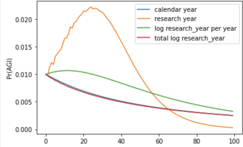
The first model, where a trial is a researcher-year, predicts a large spike of probability after a certain number of years. Here’s another diagram to illustrate this point more clearly.

 

 

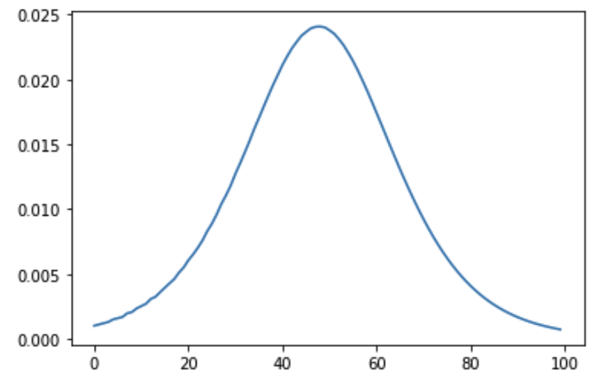
But having significantly enhanced unconditional probability in AGI happening after 50 years of research rather than 70 or 30 years doesn’t seem reasonable given my deep uncertainty, even with exponentially growing research effort. This is a reason to reject the 1st definition (trial = researcher-year).

10.4.2.3 Conditional probability curves over the time until AGI

The conditional probability of success in trial n is pr(trial n succeeds | trial 1 through trial n – 1 all fail). See more explanation here.

I plotted the conditional probabilities generated by each model, under the assumption that the number of AI researchers was growing at a constant exponential rate.

 

 

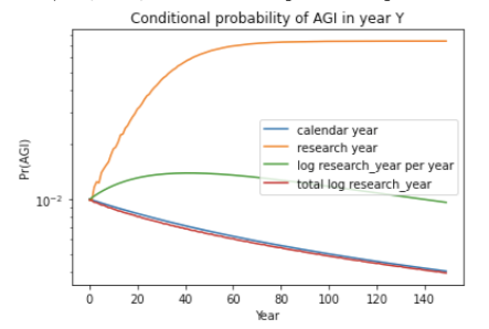
In other words, even if 1000 years of exponentially-growing sustained effort had failed to produce AGI, the first definition would remain equally confident that the next year will succeed. Even after 1 million years, it would remain just as optimistic about the next year’s prospects. I think that this behavior is unreasonable. The other two trials give more reasonable behavior.

Of course, the desired behavior could be achieved using a hyper-prior with some weight on the first definition, and some weight on other trial definitions

10.4.2.4 A shared drawback

One drawback of all the above models is that none of them explicitly model the fact that further research is evidence that previous research made good progress. The recent fast growth in the number of AI researchers is evidence of impressive progress being made, but this isn’t explicitly modeled by these definitions.

10.4.3 Derivation relating my trial definition to a model of R&D

My preferred researcher-year trial definition is ‘a 1% increase in the total researcher-years so far’. When this definition is used, the semi-informative priors framework assumes:

q: Each 1% increase in the total researcher-years so far has a constant (but unknown) probability of developing AGI.152

This appendix derives q from three assumptions discussed in the main text:

1. Ȧ = δr(t)A(t)^φ.
   • A(t) is the level of AI technological development at time t.
   • r(t) is the number of AI researchers at time t.
   • δ is a positive constant.
   • φ describes the degree of increasing (φ > 0) or diminishing (φ < 0) returns to AI R&D.
2. φ < 1.
   • This caps the degree of increasing returns to AI research.
3. Each 1% increase in A has a constant probability of developing AGI.153

10.4.3.1 Derivation

\( \dot A=δr(t)A^ϕ \, \, \, \, \, \, \, \mathrm {(Assumption \, 1)} \) \( \dot A/A^ϕ=δr(t) \) \( ∫^t_{−∞} \dot A/A^ϕ \, dt=δ∫^t_{−∞}r(t) \, dt \)

Let R(t) be the total researcher-years by time t:

\( R(t)≡∫^t_{−∞} r(t) \, dt \) \( ∫^t_{−∞} \dot A/A^ϕ \, dt=δR(t) \, dt \) \( A^{1−ϕ}/(1−ϕ)=δR(t) \, \, \, \, \, \, \, \, \, \mathrm {Assumption \, 2 \, ensures} \, φ ≠ 1 \) \( A^{1−ϕ}=(1−ϕ)δR(t) \) \( A=(1−ϕ)δR(t)^{1/(1−ϕ)} \) \( A(t)=kR(t)^m, \mathrm {with \, positive \, constants}\, k=[(1−ϕ)δ]^{1/(1−ϕ)} \ and \, m=1/(1−ϕ) \) \( \mathrm {Positivity \, of \, both \, constants \, follows \, from \, Assumption \, 2} (φ < 1) \)

If R(t) increases by 1% – a factor of 1.01 – then A(t) increases by a factor of 1.01^m. The percentage increase to A is the same for each 1% increase in R. So each 1% increase in R leads to a fixed percentage increase in A, and thus (by Assumption 3) to a fixed probability developing AGI. Hence we have deduced q.154

For example, if φ = 0.5, m = 2 and each 1% in R leads to a 2.01% increase in A, which is 2 successive 1% increases, so a fixed probability of developing AGI (by Assumption 3). More generally, each 1% increase in R corresponds to m 1% increases in A, and so to a fixed probability of developing AGI.

10.4.4 Table of results for conservative g_exp

GEXP = 4.3%		PR(AGI BY 2036)
		CALENDAR YEAR TRIAL DEFINITION	RESEARCHER-YEAR TRIAL DEFINITION
			GACT = 3%	GACT = 7%	GACT = 11%	GACT = 16%	GACT = 21%
ftpcal	1/50	12%	7.4%	11%	13%	15%	16%
	1/100	8.9%	4.5%	8.0%	10%	12%	13%
	1/300	4.2%	1.8%	3.6%	5.1%	6.5%	7.6%
	1/1000	1.5%	0.55%	1.2%	1.8%	2.5%	3.1%

10.5 Empirical data on number of AI researchers

There are a number of different estimates for the growth rate of AI researchers included below. My preferred source is the AI index 2019, which finds that the number of peer-reviewed papers has grown by 11.4% on average over the last 20 years.

• Attendance at the largest conferences increased by 21% annually between 2011 and 2018.
• In his (unpublished) article on Laplace’s law of succession, Toby Ord bounds growth of the number of researchers between 3% and 12%.
• OECD data shows total AI publications increased 9% annually from 1980 to 2019, though only 3% over the last 10 years.
• In 2019 there were 22,400 researchers published, 19% more than 2018 (source). If there were 10 in 1956 then this implies 13% growth.
• Tencent did a 2017 study concluding that there are 200,000 researchers worldwide in tech. If there were 10 in 1956, this implies 17% growth.
• AI index 2019:
  • AI’s proportion peer-reviewed papers increased 3 fold in the last 20 years, 5.7% annual growth.155
  • Absolute number rose from 10,319 to 88,429 in the same period, 11.4% annual growth.156
  • See 2018 data on p11 here.

10.6 The conjunctive model

10.6.1 Determining first-trial probability for the conjunctive model

The first-trial probability should increase with the number of conjuncts, to satisfy the constraints we used to choose its value for the non-conjunctive model.157 In particular, we need to pick a first-trial probability large enough to avoid confidently ruling out AGI in the first 100 years of trying. For reference, in my original non-conjunctive model (where there is essentially just 1 conjunct), first-trial probability = 1/300 → pr(AGI in the first 100 years of trying) = 25%.

The following plot shows how pr(AGI in the first 100 years of trying) varies with the first-trial probability for different numbers of conjuncts.

 

 

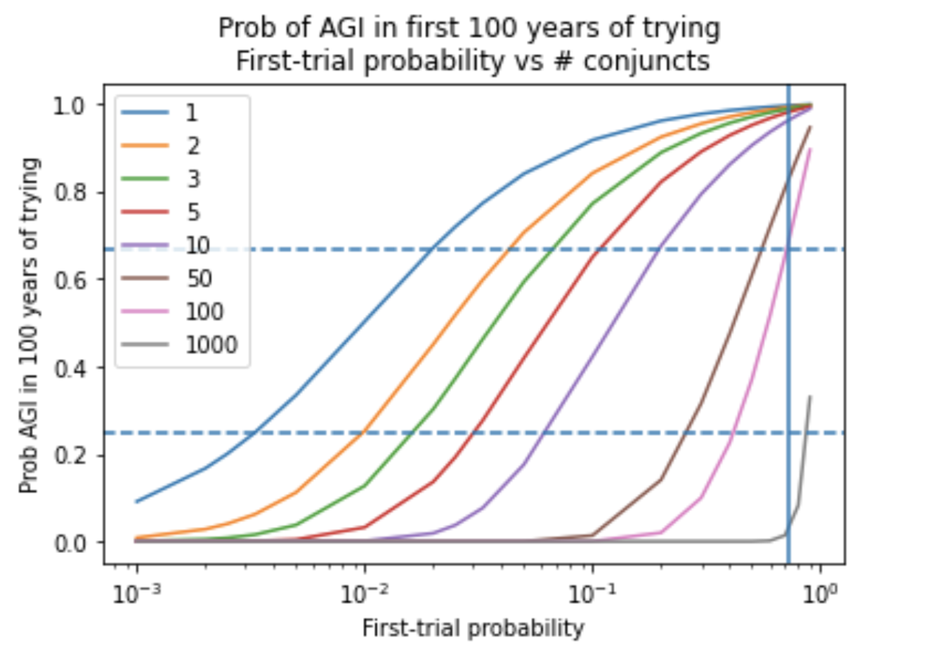
The dotted line crosses each curve at the point at which its first-trial probability is such that pr(AGI in the first 100 years of trying) = 25%. The logical widths chosen in this way are:

NUMBER OF CONJUNCTS	FIRST-TRIAL PROBABILITY
1	1/300
2	1/100
3	1/60
5	1/30
10	1/17

This is the methodology used to choose the first-trial probability for curves shown in the main text.

10.6.2 Generate low pr(AGI by 2036) with the conjunctive model

Let’s assume all conjuncts have a regime start-time of 1956 and a high first-trial probability of 0.5.158 Further assume that in 2020 we know that n independent conjuncts have still not happened after 64 years of effort. After updating on the failure to achieve each individual conjunct, you have the following beliefs:

NUMBER OF REMAINING CONJUNCTS	PR(AGI BY 2036)	PR(AGI BY 2120)
1 (i.e. standard Laplace)	20%	61%
2	4%	37%
3	0.8%	22%
4	0.2%	14%
5	0.03%	8%

The existence of just three independent conjuncts that both haven’t been achieved is sufficient to bring the bottom line down to below 1%; adding more conjuncts reduces it much further. The table shows that, despite this, the pr(AGI by 2120) isn’t that low.159

The reason is that if multiple conjuncts haven’t been achieved, we update towards each of them being hard; if they’re independent, then the chance they’re all solved soon is low. Nonetheless, there’s a chance they’ll all have time to be solved in the next 100 years.

The interesting thing about this result is that it holds no matter how many conjuncts there were to begin with. Even if there were initially 1000 conjuncts and 997 are now achieved, this model treats each conjunct as independent and so won’t infer from the 997 successes to think that the next three conjuncts will be easy. Rather, it looks at the fact that the three conjuncts have failed 60 times each and concludes they’re each hard in an uncorrelated way. This highlights how aggressive the assumption of independence is.160

Another, perhaps more plausible, way to generate smaller pr(AGI by 2036) would be to specify that multiple independent conjuncts remain, but claim we’ve only been attempting them for a short period of time (e.g. 5 years) rather than since 1956. I have not modeled this.

10.7 Why you should use a hyper-prior

Suppose you think two different update rules, r and s, are both somewhat plausible. One might define trials in terms of researcher-years, the other in terms of compute. A natural way to calculate your all-things-considered bottom line is to place some weight on both r and s. You might place 50% weight on each.

This raises a question: When you update on the failure to develop AGI by 2020, should you update the weights on these update rules? I think so. I’ll give two arguments for this. The first is a quick intuition pump. The second shows that not updating weights leads to inconsistent predictions: the probabilities you assign to an outcome depend on how you’re asked the question such that, if you make bets based on these probabilities, you’ll make a series of bets that will certainly lose you money.

10.7.1 Intuition pump for using a hyper-prior

Suppose that in front of you is a red button. God told you that he flipped a coin – if it landed heads he made it so that each press of the red button has a 80% chance of creating a popping sound; if tails then the probability would be 1%.

Before pressing the button you of course have 50% probability on the coin having landed heads. As such you have 0.5 × 80% + 0.5 × 1% = 40.5% probability that pressing the button will create a popping sound.

You press the button and there’s no popping sound. What should your probability be that the coin landed heads? And what should your probability be that pressing the button again will produce a popping noise?

Clearly, you should update towards the coin having landed on tails. Your evidence is just what you’d expect if it landed on tails, but surprising if it landed on heads. (You could use Bayes Theorem to calculate exactly what size of the update is.) As a result, your probability of the button creating a popping sound when next pressed should be lower.

The situation is analogous if you initially have 50% on two update rules, r and s. Suppose r implies that there’s an 80% chance AGI will have happened by 2020, while s implies the probability is only 1%. Our evidence (no AGI by 2020) is just what we’d expect if s is correct, but surprising if r is correct. As in the above example, we should update towards s being correct.

10.7.2 Why no hyper-prior leads to inconsistent probabilities

Let’s return to the example of a red button. For simplicity, let’s suppose r states that each press has 50% chance of creating a sound, while s states each press has 0% chance.

Alex places 50% weight on r and 50% weight on s, but he won’t update these weights over time. We’ll show that Alex generates inconsistent predictions about i) the probability that a popping sound is produced on either of the first two presses of the red button and ii) the probability that none of the first three presses produces a sound. Proof (ii) is significantly easier to follow – I recommend skipping proof (i) and going straight to proof (ii).

Note: before convincing myself of arguments (i) and (ii) I thought updating a hyper-prior was optional. In fact, I initially thought it may be better to have static weights on different priors, rather than to update a hyper-prior. This is why I took the time to write these arguments out in full. However, it may be obvious to some readers that we have to update a hyper-prior, and arguments will be overkill.

10.7.2.1 i) What’s the chance that 1 of the first two presses makes a sound?

Some terminology will be useful.

• f = the first press of the red button produces a sound
• s = the second press of the red button produces a sound
• b = both the first and second presses of the red button produces a sound. We’ll ask Alex two sets of questions, and he’ll predict different values for his all-things-considered pr(b) each time.First set of questions – ask what pr(b) is according to each theory and combine the results.
  1. Conditional on r being correct, what is pr(b)? The answer is 1/4.
  2. What is the chance that r is correct? The answer is 1/2.
  3. Conditional on s being correct, what is pr(b)? The answer is 0.
  4. What is the chance that s is correct? The answer is 1/2.

  The all-things-considered pr(b) can be deduced from these answers. pr(b) = 1/4 × 1/2 + 0 × 1/2 = 1/8.

  Second set of questions – ask what pr(f) and pr(s | f) are separately, each time using the first set of questions. Then combine the results.

• What’s the all-things-considered pr(f)? The answer is 1/2 × 1/2 + 0 × 1/2 = 1/4.
  1. Conditional on r being correct, what is pr(f)? The answer is 1/2.
  2. What is the chance that r is correct? The answer is 1/2.
  3. Conditional on s being correct, what is pr(f)? The answer is 0.
  4. What is the chance that s is correct? The answer is 1/2.
• What’s the all-things-considered pr(s | f)? The answer is 1/2 × 1/2 + 0 × 1/2 = 1/4.
  1. Conditional on r being correct, what is pr(s | f)? The answer is 1/2.
  2. What is the chance that r is correct? The answer is 1/2.
  3. Conditional on s being correct, what is pr(s | f)? The answer is 0.
  4. What is the chance that s is correct? The answer is 1/2.

The all-things-considered pr(b) can be deduced from these answers. pr(b) = 1/4 × 1/4 = 1/16.

So Alex has given inconsistent answers. If he made bets about the various sub-questions, he could be Dutch-booked. If he had updated his weights, he’d have avoided this. In this case, the all-things-considered pr(b) couldn’t be deduced from our first four questions, as our probability that r is correct changes over time. So only the second method would be valid (although the answer to question 6 would change) and the contradiction could be avoided.

We can create a similar paradox in the case of AGI timelines with the following definitions:

• f = we won’t develop AGI in 2021
• s = we won’t develop AGI in 2022
• b = we won’t develop AGI in 2021 or 2022

Someone with static weights over different update rules will give different predictions for pr(AGI by 2022) depending on whether they i) calculate pr(AGI by 2022) for each rule separately and then take the average, or ii) take a weighted average to calculate pr(AGI by 2021), and then take a weighted average to calculate pr(AGI by 2022 | no AGI by 2021). Methods i) and ii) correspond to the first and second sets of questions we asked Alex above.

I believe this argument is a special case of the general argument in favor of updating your probabilities in accordance with Bayes’ theorem when you receive new evidence.

10.7.2.2 ii) What’s the chance that any of the first three presses makes a sound?

Remember, r states that each press has 50% chance of making a sound, while s states each press has 0% chance. Alex places 50% weight on r and 50% weight on s, but he won’t update these weights over time.

Alex thinks that there’s 50% that pressing the button will never make a sound. For he places 50% weight on s, which implies this.

However, if you sum up the probability that Alex assigns to any of the first three presses making a sound, it’s greater than 50%. He calculates the first press has 50% × 50% = 25% probability of making a sound. He doesn’t update his weights, so calculates the second press also has 50% × 50% = 25% probability. Similarly, he will judge the third press to have a 25% chance of making a sound. This implies that the chance that none of the first three presses makes a sound is 0.75 × 0.75 × 0.75 = 42%, and so 58% chance that one of the initial presses makes a sound. So Alex’s probabilities are inconsistent.

So on one method the probability is 50%, on another it’s 58%.

The problem is that Alex should increase his confidence in s if the first press doesn’t make a sound. He should update his weights.

A similar counterexample can be constructed if r is a Laplace prior over whether each press will make a sound, and s is again the view that the button cannot produce a sound.161

10.8 Investigation into using a hyper-prior on updates rules with different trial definitions

Suppose you initially have equal weight on multiple update rules that have different trial definitions. What is the effect of hyper prior updates?

In my investigation I placed 50% weights on two update rules. I looked at how these weights changed by 2020, and the effect on the bottom line.

The first update rule always had the following inputs:

• Trial definition: calendar year
• Regime start-time: 1956
• First-trial probability: 1/300

I varied the second update rule.

Each row in the following table corresponds to a different second update rule. The table shows the inputs to this second update rule, the effect of hyper prior updates on pr(AGI by 2036), and how much the weight on the second update rule changed from its initial value of 50%. I assume aggressive compute spend where applicable.

2ND UPDATE RULE INPUTS			PR(AGI BY 2036)		WEIGHT ON SECOND RULE IN 2020
TRIALS DEFINED USING…	FIRST-TRIAL PROBABILITY162	REGIME START-TIME	STATIC WEIGHTS	HYPER PRIOR UPDATES
Researcher- years	Medium: gexp = 4.3% gact = 11%	1956	6.1%	5.9%	44%
Researcher- years	High: gexp = 4.3% gact = 21%	1956	7.6%	6.8%	38%
Researcher- years	High: gexp = 4.3% gact = 21%	2000	9.9%	9.7%	48%
Compute	Medium: gexp = 4.3% X = 5	1956	8.4%	7.8%	43%
Compute	High: gexp = 4.3% X = 1	1956	13%	8.3%	23%
Compute	Lifetime learning hypothesis	1956	10%	8.6%	38%
Compute	Evolution compute hypothesis	Very late163	13%	14%	55%

When the regime start-time is 1956, the hyper prior updates tend to bring the overall bottom line down in the 5 – 10% range, but not below that. However, with late regime start-times, hyper prior updates have very little effect and the bottom line can remain above 10%.

Here’s a slightly more detailed summary of the patterns in the above table and in the table in the main text:

• Hyper prior updates reduce pr(AGI by 2036) compared with having static weights, but not by much. The reduction is greater if there’s initially significant weight on update rules with wide-ranging annual probabilities.
• If your overall bottom line is >10%, hyper prior updates reduce it into the 5 – 10% range.
• If your overall bottom line is in the 5 – 10% range, hyper prior updates might reduce it by ~2%.
• If your overall bottom line is below 5%, hyper prior updates have a negligible effect.164
• If you have a late regime start time, hyper prior updates have a negligible effect.

10.9 Investigation into ‘AGI is impossible’

In my investigation I considered a variety of update rules that we’ve seen in this report. For each update rule U, I looked at its pr(AGI by 2036) when I assigned 0% and 20% initial weight to ‘AGI impossible’ and the rest of my initial weight to U. I also looked at how much the weight assigned to ‘AGI impossible’ had increased by 2020 from its starting point of 20%. I assume aggressive compute spend where applicable.

UPDATE RULE INPUTS
TRIALS DEFINED USING…	FIRST-TRIAL PROBABILITY	REGIME START-TIME	INITIAL WEIGHT ON ‘AGI IS IMPOSSIBLE’
			0%	20%
			PR(AGI BY 2036)	PR(AGI BY 2036)	WEIGHT ON ‘AGI IS IMPOSSIBLE’ IN 2020
Calendar year	Medium: 1/300	1956	4.2%	3.2%	23%
Researcher- years	Medium: gexp = 4.3% gact = 11%	1956	7.9%	5.7%	28%
Researcher- years	High: gexp = 4.3% gact = 21%	1956	11%	7.3%	33%
Researcher- years	High: gexp = 4.3% gact = 21%	2000	16%	12%	25%
Compute	Medium: gexp = 4.3% X = 5	1956	13%	8.9%	29%
Compute	High: gexp = 4.3% X = 1	1956	22%	11%	50%
Compute	Lifetime anchor	1956	16%	11%	38%
Compute	Evolutionary anchor	Very late	22%	17%	22%
Compute	Log-uniform	Very late	28%	22%	22%

10.10 Objections and replies

10.10.1 The model unrealistically assumes that AI R&D is a series of Bernoulli trials

It is true that a more realistic model would allow for the fact that AGI will be produced sequentially in many stages that each builds on previous progress, and it is true that this lowers the probability of creating AGI in very early trials.

I give three responses to this objection.

My first response is that this problem can be partly avoided by choosing a later regime start-time. The sequential nature of AGI development does indeed mean that the unconditional annual probability of developing AGI is very low in the very first years of effort. However, my deep uncertainty about how hard AGI may be to develop means it shouldn’t stay very low for too long. For example, it shouldn’t still be low 30 years after 1956. We can delay the regime start-time so that it occurs once enough time has passed that the annual probability of developing AGI is not too low. For example, if you think the field of AI R&D had no chance of success in the first 10 years, but might have succeeded after this point, then your regime-start time can be 1966.

This response is not fully satisfactory. A limitation is that the probability would not suddenly jump up from 0 in 1966, but rise slowly and smoothly. Further, after 1966 the sequential nature of development might still affect the shape of the probability distribution, making it different from the probability distribution of my model.

My second response is to suggest that people with this worry adapt their non-conjunctive models by converting them into a conjunctive or sequential model as described here. The conjunctive model explicitly acknowledges that multiple distinct tasks have to be completed to achieve AGI, the sequential model additionally requires them to be completed one after the other. This implies a very low probability of success in initial trials which then rises after a few decades.

These models give similar probabilities to the equivalent non-conjunctive model (within a factor of 2) after 20 – 50 years of R&D.165 The reason for this is that they remain agnostic about the proportion of conjuncts that have been completed. After a few decades, they assign weight to there only being a few conjuncts remaining, and so make similar predictions to non-conjunctive models.

My third response is that when I defend the adequacy of this framework, I focus on the family of unconditional distributions over trials that the Bernoulli model gives rise to. I argue that using a different family of distributions wouldn’t significantly change the bottom line. If this is correct, it does not matter if they were derived from an unrealistic assumption. This side-steps the question of whether Bernoulli trial model is accurate.

I discuss this objection at greater length in my reply to the review by Alan Hajek and Jeremy Strasser (see here).

10.10.2 This framework would assign too much probability to crazy events happening

Would this framework assign too much probability to the Messiah coming each year, or us finding the philosopher’s stone? I don’t think so.

If we apply the framework to crazy events like these, there should be some significant differences in the inputs that we use. These will include some of the following, all of which lower pr(crazy event by 2036):

• Lower first-trial probability. The moderately-sized first-trial probability for AGI was driven by AGI being a central aim of a serious STEM field. This isn’t currently true of the crazy events offered as examples above, so there wouldn’t be reason to assign them a comparably high first-trial probability as AGI.
• Earlier regime start-time. People have been looking for the elixir of life, and trying to turn lead into gold, for a long time. This might justify early regime start-times.
• Higher initial weight on impossibility. Most experts regard AGI as feasible in principle, and many think it may be feasible in the next few decades. In addition, a human is an existence proof for a generally intelligent system. These considerations suggest the initial weight we should assign to ‘AGI is impossible’ should be fairly small. Such considerations typically do not apply for other crazy events people apply the framework to.
• Predict ‘time when the occurrence of X is predictable’ rather than ‘time when X’. Some events will have clear precursors. In this case, the semi-informative priors framework is more usefully applied to predict when these precursors will first become apparent,166 as we can typically rule out the event in the near future based on the lack of precursors. For example, it wouldn’t be useful to predict ‘time until Mars is colonized’ using this framework, as we can rule out such colonization in the near future based on the lack of precursors and so the framework’s predictions would be substantially changed by this additional evidence. It might, though, be useful to predict ‘time until unambiguous signs are present about when we will colonize Mars’ using this framework.
• Different R&D inputs. The number of AI researchers, and the amount of compute used to develop AI systems is currently growing very quickly. This drives the probabilities of the report upwards. For many other ‘crazy’ events or developments, the resources being used to pursue them is lower than at previous times. Using trials defined in terms of these inputs would lead to much lower probabilities.

When constraining the first-trial probability for AGI I explicitly considered whether my reasoning might lead to implausible predictions when applied to other R&D efforts (here). I concluded that a first-trial probability larger than 1/100 might lead to implausible results, but could not give a good argument for thinking values lower than 1/100 would do so.

10.10.3 Is the framework sufficiently sensitive to changing the details of the AI milestone being forecast?

Suppose that, instead of forecasting AGI, this report was forecasting ‘chess grandmaster AI’, or ‘superintelligent AI’. Would it make similar predictions? If so, that seems to be a problem.

The only way the framework could make different predictions about other AI milestones is if I used different inputs. In particular, the first-trial probability (ftp) and the initial weight on impossibility are the two inputs most likely to make a significant difference. So it all depends on how the inputs are selected, and how sensitive this process is to the specific milestone being forecast. It is less a question of the framework, and more on how the framework is being applied. In principle the framework could be highly sensitive, or highly insensitive, to differences in the milestone being forecast.

In the case of this report, my methods are somewhat sensitive to the specific milestone forecast. The milestone influences the reference classes we use to constrain ftp and the weight we place on these reference classes. For example, the reference class ‘transformative technological development’ would be inappropriate for ‘chess grandmaster’, and the reference class ‘feasible technology that a serious STEM field is explicitly trying to build’ would be less relevant to ‘super intelligent AI’ than to ‘AGI’.

However, the report’s methods for choosing the inputs require highly subjective judgment calls. These judgments may not be sensitive to minor changes in the milestone being forecast. Even for major changes in the milestone, the way the inputs change will be highly subjective.

10.10.4 This framework treats inputs to AI R&D as if they were discrete, but in fact they are continuous!

The inputs to AI R&D studied in this report are time, researcher-years, and compute. All these quantities are clearly continuous. Yet my framework divides them into “chunks”, with each chunk corresponding to a trial. Wouldn’t it be better to use a continuous framework, to match the continuous nature of the inputs?

Indeed, it would be theoretically cleaner to use a continuous framework. I do not do so for two reasons. Firstly, I find the discrete framework to be simple to explain and understand, and easy to work with.

Secondly, and more importantly, I am confident that the results would not change if I took this framework to its continuous limit. As discussed in Section 3.2.2, the predictions of the framework do not materially change if we change the trial definition from (e.g.) 1 year to 1 month.167 In fact, throughout this report I subdivide trials into very small parts to ensure none of the results are a product of an unrealistic discretization of effort. For example, although the report defines a researcher-year trial as ‘a 1% increases in total researcher-years so far’, my calculations use a 0.01% increase instead.

The subdivisions are small enough that subdividing further makes no difference to any of the results displayed in the report. For this reason, I am confident that taking the framework to the continuous limit would make no difference to the results (the continuous limit is simply what you get when the size of the subdivisions tends to 0).

10.11 How might other evidence make you update from your semi-informative prior?

This report aims to arrive at a semi-informative prior over AGI timelines, which roughly means:

What would it be reasonable to believe about AGI timelines if you had gone into isolation in 1956 and only received annual updates about the inputs to AI R&D and the binary fact that we have not yet built AGI?

What kinds of evidence might update you on this semi-informative prior, and how might it cause you to update? Rather than trying to be comprehensive, I just briefly outline a few possibilities, to give a sense of how a semi-informative prior can be adjusted to get closer to an all-things-considered view.

State of the art AI systems aren’t collectively almost as capable as AGI. Though we have systems that outperform humans in many narrow domains, and some systems show potential signs of generality, there are still many domains in which AI systems are not close to matching human performance. For example, tasks like “being a good parent”, “running a company”, “writing a novel”, “conducting scientific research”. Although current progress is fast, it doesn’t seem it’s so fast that we’ll reach systems this capable in the next few years. This consideration should update you away from AGI happening in the next few years, compared to this report. Exactly how strong this update is, and how long into the future it lasts, depends on a few things: i) how large you think the gap is between today’s systems and AGI, ii) how slowly you think today’s systems are currently improving, iii) how steady you expect the rate of progress to be over time, iv) how confident you are in judgments (i), (ii) and (iii).

Expert surveys.168 These assign higher probabilities to success in the coming decades than the probabilities from this report. If you trust these surveys, you should increase your probabilities towards those offered in the surveys. The more you trust them, the larger the update.

Alternative frameworks for forecasting AGI timelines. My colleague Ajeya Cotra has written a draft report on how much compute it might take to train a transformative AI system, and when this amount of compute might be affordable. She assigns slightly higher probabilities to developing AGI in the coming decades to this report. If you find the report convincing, you should update your probabilities towards those offered by the report.

Economic trends. In many models of machine intelligence, development of systems like AGI that can allow capital to effectively substitute for human labour can lead to increases in the economic growth rate.169 If there are reasons from economics to doubt that such an increase is likely to occur – for example the striking consistency of US GDP/capita growth over the last 150 years – this may reduce the probabilities of AGI from this report. On the other hand, many models extrapolating long-run GWP data predict the growth rate to increase significantly over the 21st century – for example see Lee (1988), Kremer (1993) and Roodman (2020). If these models are given sufficient weight, economic considerations might increase the probabilities from this report. I plan to publish a report assessing these economic considerations in the near future.

In general, the more confident you are in types of reasoning like the above, the less you will lean on this report’s conclusions.

10.12 Is the semi-informative priors framework sufficiently expressive?

This section is quite heavy on mathematics and doesn’t have any implications for the bottom line. It’s probably only worth reading in full if you want to understand the generality and potential limitations of the mathematical framework used in this report.

The family of update rules I’ve looked at model the AGI development process as a series of ‘trials’ where each trial has a constant but unknown probability p of creating AGI.170 So far, the report has mostly focussed on how E(p) – our estimate of the probability of success on the next trial – changes over time. E(p) is our conditional probability that the next trial succeeds, given that all previous trials failed.

However, you can derive our unconditional probability distribution P(n) that trial n will be the first in which AGI is created. This is what you should believe before the regime start-time, when you know nothing about the failure of any of the trials. In this section I’ll call any such P(n) you can generate with different inputs a semi-informative distribution over the trial in which AGI will be created. It turns out the family semi-informative distributions are known as beta-geometric distributions.

More formally, P(n) = pr(the first success occurs in trial n) = pr(trial 1 fails & trial 2 fails &… trial n-1 fails & trial n succeeds). It is the subjective probability distribution of someone who knows that each trial has a constant but unknown probability p of success, initially represents their uncertainty about p with a Beta distribution, and anticipates updating this subjective probability distribution over p in response the outcomes of observed trials (in accordance with the requirements of Bayesian inference).171 The exact form of P(n) depends on the first-trial probability and the number of virtual successes (I give a formula for a special case below).

Although P(n) follows in this way from the assumption of repeated trials with constant but unknown probability of success, we equally could take P(n) to be a primitive of the framework. We would divide AI inputs (time, researcher-years, compute) into chunks and talk directly about our unconditional probability that AGI is created in each chunk: P(n) = pr(chunk n of input is the first to lead to AGI). We would think of P(n) as directly expressing our distribution over the amount of R&D input (time / researcher-years / compute) required to develop AGI (having discretized the input into chunks). This would eliminate talk of ‘trials’, ‘updates’, and ‘our distribution over p’. From this perspective, the framework is not Bayesian as we do not update our belief about any parameter. We simply specify inputs (first-trial probability, virtual successes) to determine a probability distribution over the total time / researcher-years / compute required to develop AGI. (Of course, from this perspective the choice of beta-geometric distributions is unmotivated.)

This is the perspective adopted in this section. I take the distributions P(n) to be primitive entities of the semi-informative priors framework, and ask whether considering alternative distributions would shift our bottom line by much. To this end, I do the following:

• Give a simple formula for P(n) in the special case with 1 virtual success, and plot how P(n) depends on key inputs (here).
• Describe how P(n) relates to how other popular distributions and explain why I don’t use those distributions (here).
• Give a quick intuitive explanation for why I don’t think other distributions would change the bottom line by more than 2X (here).
• Outline a more detailed (but still inconclusive) argument for why other distributions wouldn’t significantly change the bottom line (here).
• Recap some limitations of this framework (here).

10.12.1 Formula for P(n)

If there’s one virtual success, the unconditional probability that AGI is created in trial n is:

\( P(n)≃β/(β+n)^2 \)

Where β = (1 / first trial probability) – 1 is the number of virtual failures. When there’s 1 virtual success, β is also the median number of trials you initially expect it to take to build AGI. In Laplace’s rule of succession, β = 1 ; I prefer a first-trial probability of 1/300, which implies β = 299.

The approximation in the formula holds closely when β + n > 10 (see more detail about P(n) in this appendix). To be clear, this equation does not define P(n); it is a formula for calculating its value when there’s 1 virtual success; the definition of P(n) was given in the previous section.

If β is small P(n) starts high but falls off quickly (~1/n²). If β is large then P(n) starts lower but initially falls off very slowly. P(n) is a quarter of its initial value when n ≃ β.172

I produced plots of how the first-trial probability and number of virtual successes affect the shape of P(n).

 

 

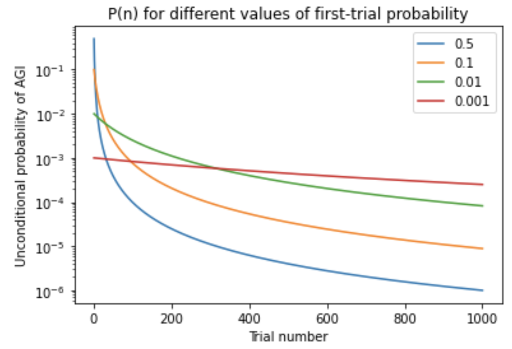
Notice that every line starts at its first-trial probability, and that the larger this is the quicker P(n) falls off. It is not surprising that the lines cross, they must do so for P(n) to sum to 1 across all n.

 

 

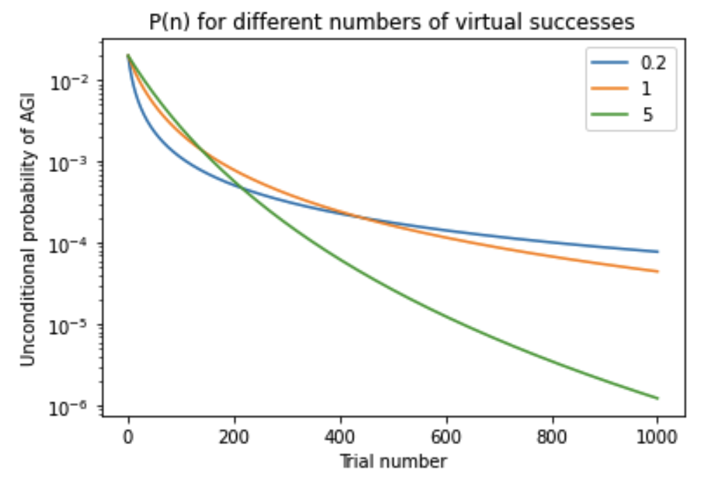
Notice that the number of virtual successes controls how quickly the probabilities fall off in the tail.

Remember to distinguish the above graphs of unconditional probabilities from the conditional probability of success in the next trial given that all previous trials have failed (I discuss the difference here). The conditional probability, which we’ve referred to as E(p), is discussed here. The following graphs show how this depends on the first-trial probability and number of virtual successes.

 

 

 

 

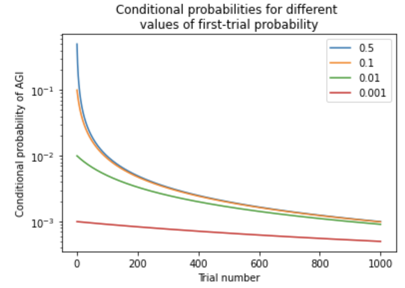
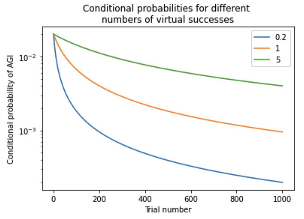
It is the unconditional probabilities P(n) that I focus on in this section here.

10.12.2 Relation of framework to other distributions

I explain how semi-informative distributions P(n) compare to some commonly used distributions:

• Pareto
• Geometric
• Uniform
• Normal

All distributions are understood as distributions over the total amount of input (time / researcher-years / compute) required to develop AGI.173

The first two are special instances of the framework, the second two are not. My favored inputs don’t approximate any of these distributions, for reasons that I explain below.

10.12.2.1 Pareto

10.12.2.1.1 Semi-informative distributions can express Pareto distributions

Fallenstein (2013) places a Pareto distribution, sometimes referred to as a power law, over the total time until AGI is developed. We could also imagine placing a Pareto distribution over researcher-years or compute required for AGI (or over the log(researcher-years) and log(compute) required, as this report favors).

The probabilities implied by this use of a Pareto distributions are a special case of the semi-informative distributions.

Pareto distributions have two parameters:

• x_m is the minimum possible value of x.
  • In this context, it gives the amount of time that we’ve been trying to build AGI but not succeeded.174
• α controls how likely x is to be close to x_m; the larger α the more likely x is to be close to x_m. (For example, Pr(x_m < x < 2x_m) = 1 – α/2.)

This Wikipedia diagram shows some examples for x_m = 1:

 

 

Pareto is continuous, but it is very natural to discretize it as follows:

1. Interpret Pr(n – 1 < x < n) as the probability that AGI is created on trial n.
2. Force x_m to be an integer. x_m then gives the number of failed trials.

With this discretization, the probabilities from a Pareto distribution are identical to those from a semi-informative distribution with the following parameters:

• The number of virtual successes = α.
• The first-trial probability is chosen so that probability of success in the trial x_m + 1 (i.e. the first trial that the Pareto distribution doesn’t assume has failed) equals that of the Pareto distribution.
• First, calculate z = Pr(x_m < x < x_m + 1) according to Pareto.
• Second, choose the first-trial probability so that pr(success in the (x_m + 1)th trial | trial 1 through trial x_m all fail) = z.175

With these parameters you find the Pareto Pr(x_m + n – 1 < x < x_m + n) is equal to the semi-informative pr(AGI in trial x_m + n | trials 1 through trial x_m all fail), for all positive integers n. I know this because I demonstrated the result in simulation; I have not proven it analytically.176

This result should not be surprising given that Pareto distribution with α = 1 is the continuous limit of Laplace’s rule of succession. I believe, but have not formally derived, that all Pareto distributions are the same as the continuous limit of some semi-informative distribution.

10.12.2.1.2 All semi-informative distributions approximate Pareto distributions in the tail

Take any semi-informative distribution, with number of virtual successes = v and first-trial probability = 1/γ. After updating on a sufficiently large number of failed trials n, its probability distribution over remaining trials closely approximates that of a Pareto distribution. In other words, semi-informative distributions have power-law tails.

In particular, once n/v ≫ γ, its probability distribution over remaining trials closely approximates that of a Pareto distribution with x_m = n and α = v. An intuitive way to understand the mathematical condition n/v ≫ γ is that the semi-informative distribution has entered its tail.

(For comparison the conditional probability pr(success in trial n | trials 1 through n-1 fail) = E(p) = 1 / (γ + n/v). When n/v ≫ γ, this simplifies to E(p) = v/n. In the limit the relevance of the first-trial probability disappears.)

As above, I did not prove this result analytically, but demonstrate it in simulation.177 The following diagram shows the approximation for various values of n for the standard Laplace distribution (1 virtual success and first-trial probability = 1/2).

 

 

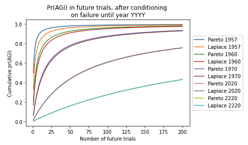
Here N is the number years since the regime-start time in 1956. By 1970 (n = 14) the approximation is very good, and by 2020 the curves are almost indistinguishable.

10.12.2.1.3 How my favored inputs differ from Pareto

Although the semi-informative priors framework can express Pareto distributions, I don’t put significant weight on inputs that approximate Pareto over the next few decades. Why is this?

Pareto distributions have the following ‘scale invariance’ property:

\( Pr(X<cx|X>x)=Pr(X≤cy|X>y), for \, all \, x, y, c>1 \)

In other words, the answers to the two following questions are the same:

1. If we’ve had 20 years of effort without developing AGI, what’s the chance of success in the next 20 years?
2. If we’ve had 30 years of effort without developing AGI, what’s the chance of success in the next 30 years?

(This example uses x = 20, y = 30, c = 2, and takes trials to be calendar years.)

This property might seem intuitive, but it is unreasonable near the regime-start time. To see this, let x = 1, y = 30, and c = 2. Then it says the following two have the same answer:

1. If we’ve had 1 year of failed attempts to develop AGI, what’s the chance of success in the next year?
2. If we’ve had 30 years of failed attempts to develop AGI, what’s the chance of success in the next 30 years?

But the first probability is much lower as we should have guessed AGI would probably be hard to create even before we started trying. To equate (3) and (4) is to make the same mistake as Laplace’s prior: assuming the only reason for skepticism is the failure of efforts so far, and ignoring our knowledge that ambitious R&D efforts rarely succeed in a small number of years.

My preferred inputs avoid this unreasonable implication by having a low first-trial probability that dampens the probabilities in early trials compared to Pareto.

Nonetheless, Pareto’s ‘scale invariance’ property will still approximately hold in the tail of all semi-informative distributions. And it should hold the tail – at this point the main reason we have for skepticism is the failure of efforts so far as (being in the tail) it’s taken much more effort than we initially expected. In other words, although semi-informative distributions are not power-law distributions, they approximate a power-law in the tail and this behavior seems reasonable.

10.12.2.2 Geometric distribution

The geometric distribution, a special case of the negative binomial distribution, is the discrete analogue of the exponential distribution.

10.12.2.2.1 Semi-informative distributions can express geometric distributions

Geometric distributions have one parameter p_o, which is the known probability of success in each trial. The following Wikipedia diagram shows the distribution for three values of p_o.

 

 

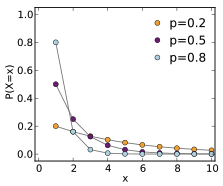
The geometric probability distribution is the limiting case of the semi-informative distribution where:

• The first-trial probability = p_o.
• We take the limit as the number of virtual successes tends to infinity. In practice you can just use a large number (e.g. 1 million virtual successes).

Proof:

Let’s consider the formula for pr(trial n succeeds | trial 1 through trial n – 1 fail).

In a geometric distribution, this quantity is constant: pr(trial n succeeds | trial 1 through trial n – 1 fail) = p_o.

In the semi-informative priors framework, this quantity is:

\( E(p)=1/(γ+N/α) \)

where γ= 1/first-trial probability, and is the number of virtual successes.

As α → ∞, E(p) → 1/γ. This is identical to a geometric distribution if p_o = γ = 1/first-trial probability. Intuitively, in this limit we already have so many virtual observations that further observed failures don’t shift our estimate of E(p) at all. Our estimate of pr(trial n succeeds | trial 1 through trial n – 1 fail) no longer depends on n and so we approximate a geometric distribution.

10.12.2.2.2 How my favored inputs differ from geometric distributions

Although the semi-informative priors framework can express geometric distributions, I don’t favor inputs that do so. In particular, I favor 0.5 – 1 virtual successes rather than ~infinite virtual successes. Why is this?

When you observe many failed attempts to develop AGI, it is appropriate to update towards thinking AGI will be harder to develop than you previously thought. In other words, pr(trial n succeeds | trial 1 through trial n – 1 fail) should decrease with n, once n is large enough.

This is most clear in an extreme case where, despite a sustained effort, we fail to create AGI in the next 10,000 years. Though I think it’s reasonable to have a prior annual probability of success of 1/300, this wouldn’t still be reasonable after 10,000 years of failed effort. But if we used a geometric distribution, then even after 10,000 years of failed effort our pr(AGI is developed in the next year) would not change. In other words, according to a geometric distribution pr(trial 10,001 succeeds | trials 1 through 10,000 fail) = pr(trial 5 succeeds | trials 1 through 4 fail), but according to my favored semi-informative distributions the latter is much higher.

10.12.2.3 Uniform distributions

10.12.2.3.1 Semi-informative distributions can’t approximate uniform distributions

In uniform distributions the unconditional probability of success on each trial between a start point and an end point is constant. By contrast, the unconditional semi-informative distribution P(n) always decreases over time for two reasons: i) later trials only happen if earlier trials fail, so are at a disadvantage, ii) by the time later trials happen we have updated towards thinking the task is harder and so think they are less likely to succeed even if they happen.

How quickly does P(n) decrease? Let’s take the case with 1 virtual success. In this case, it turns out that by the time the cumulative probability of success is 50%, P(n) has reduced by a factor of 4.178 So P(n)decreases significantly during any period where there’s a large cumulative chance of success. Over such a period, P(n)is not even approximately uniform.

10.12.2.3.2 Uniform distributions are only appropriate when we have an end-point

The constant per-trial probability of a uniform distribution is determined by the distance between the start-point and end-point. In this context, an end-point is a time by when we can be confident that AGI will have been developed.

If your end-point is arbitrary, your per-trial probability will be arbitrary. In addition, your per-trial probability will suddenly drop to 0 at the end-point. For these reasons, you should only use a uniform distribution if you have an end-point.

For most of this document I have speculated about start-points (the regime start-time) but not about end-points, and so uniform distributions haven’t been appropriate.

The only exception was when I entertained the supposition that AGI was likely to have been created by the time we had used evolution compute179 to develop an AI system (here). Here I used log-uniform distribution over the amount of development compute. I explain in this appendix why I think a semi-informative distribution isn’t appropriate when we have an end-point.

10.12.2.4 Normal

My framework cannot model a normal distribution, but I think such a distribution would be unreasonable. The tails of normal distributions fall off super-exponentially. This means that (in the tail) the longer AGI takes longer to develop, the more confident you become that the next trial will succeed.180 But this behavior is unreasonable. If we haven’t developed AGI after 500 years of sustained effort, we should not become increasingly confident that we’ll succeed each year.

A log-normal distribution over researcher-years or compute could potentially be a reasonable choice, if we have an endpoint to justify the tail falling off super-exponentially.

10.12.3 Why I suspect that using another framework wouldn’t significantly change the bottom line

The results in this document have been largely driven by i) my prior view about how hard AGI is to make and ii) my view about how to update from the fact AGI hasn’t happened yet, iii) empirical forecasts about how much inputs to AI R&D will increase by 2036.181 In other words, the results have not been driven by the specific framework I have been using, but by my choice of inputs to that framework.

Suppose we used another framework but kept our views about factors (i), (ii), and (iii) constant. I expect the new framework’s bottom line pr(AGI by 2036) would change by less than a factor of 2. A new framework would probably change the shape of the curve P(n) in various ways, for example making it slope slightly upwards rather than slightly downwards between 2020 and 2036 or changing the ratio of the gradients at different points. However, I don’t think these changes would significantly change the area under the curve between 2020 and 2036 because factors (i), (ii) and (iii) have a very significant influence on the height of the curve and we are supposing that they are held fixed. Or to take another perspective, imagine that when we move to another framework we hold fixed pr(AGI in the first 100 years). Reasonable curves that adequately express our deep ignorance but hold (i), (ii) and (iii) fixed won’t differ by more than 2X on the area under the curve between 2020 and 2036 given this constraint.

The conjunctive model is an example of a framework like this. It significantly changes the shape of the curve, moving probability mass from the early years of effort to later years. Nonetheless, when we held (i), (ii) and (iii) fixed and moved to the conjunctive model, we found that pr(AGI by 2036) changed by less than a factor of 2.

The only exception I can think of is if some framework picked out 2020-36 as a period of significantly enhanced or dampened probability of AGI. From the perspective of this project, which aims to address AGI timelines from a position of deep uncertainty, I don’t think this would be reasonable. For example, I don’t think it would have been reasonable in 1956 to say “If AGI happens in the 21st century then it’s particularly (un)likely to happen between 20XX and 20YY”.

10.12.4 A weak argument that the semi-informative priors framework is sufficiently general

The structure of this argument is as follows:

1. The framework can specify the starting value of P(n).
2. The framework is sufficiently flexible about how P(n) changes initially.182
3. The framework is sufficiently flexible about how P(n) changes in the tails.
4. Given 1-3, a different framework wouldn’t significantly change the starting value of P(n), how it changes initially, or how it changes in the tails. So a different framework wouldn’t significantly affect the bottom line.

Claim (1) is trivial – we specify P(1) directly with the first-trial probability.

The rest of this section defends 2 – 4 in turn. I think claim (4) is the most debatable. If you were convinced by the argument in the previous section, I’d skip to the next section.

10.12.4.1 The framework is sufficiently flexible about how P(n) changes initially

We saw earlier that with 1 virtual success P(n) falls off with 1 / (m + n)². However, there are other mathematical possibilities. I divide these into three camps: i) P(n) initially decreases faster, ii) P(n) initially decreases more slowly, or iii) P(n) initially increases (and then start to decrease after a bit).183

For each of these three possibilities, I find that either the framework can model the possibility, the possibility has a negligible effect on the bottom line, or the possibility is unreasonable.

10.12.4.1.1 We can make P(n) decrease as fast as we like

If we decrease the number of virtual successes P(n) initially decreases more quickly. There’s no limit to how fast we can make P(n) decrease initially. So the framework is adequately expressive in this regard.

10.12.4.1.2 We can make P(n) decrease somewhat slower

If we increase the number of virtual successes , P(n) initially decreases more slowly. There is a limit to how slowly we can make P(n) decrease initially. In the limit where the number of virtual successes tends to infinity, P(n)approaches a geometric distribution and P(n) still decreases with n.

How much difference would it make to the bottom line if we could make P(n) decrease even more slowly? The following table shows pr(AGI by 2036) conditional on it not happening by 2020 for i) a semi-informative distribution with 1 virtual success, ii) a geometric distribution, and iii) a uniform distribution with constant P(n) = P(1). All three distributions agree about the first-trial probability P(1).

	PR(AGI BY 2036)
P(1) – FIRST-TRIAL PROBABILITY	NUMBER OF VIRTUAL SUCCESSES = 1	GEOMETRIC DISTRIBUTION (NUMBER OF VIRTUAL SUCCESSES → ∞ )	PR(AGI BY 2036) – P(N) DOESN’T DECREASE, P(N) = P(1)
1/100	8.9%	15%	16%
1/300	4.2%	5.2%	5.3%
1/500	2.8%	3.15%	3.20%
1/1000	1.5%	1.59%	1.60%

Only the probabilities in the final column cannot be expressed by the semi-informative priors framework. This shows that, given that the first-trial probability < 1/100, allowing P(n) to decrease more slowly than this framework permits wouldn’t significantly change the bottom line.184 So the framework is adequately expressive in this regard.

In any case, I explained above that I don’t put much weight on inputs that approximate a geometric distribution: P(n) should decrease somewhat over time.

10.12.4.1.3 P(n) can’t increase over trials, but we can make adjustments to accommodate this

A semi-informative distribution can’t model the possibility that P(n) is higher for later trials.

I can think of two good reasons to think the unconditional probability might rise:

1. Very early trials are at a disadvantage because there’s not time to complete all the steps towards building AGI. For example, AGI was more likely to happen in 1970 than in 1957.
2. AGI is more likely to happen in 2030 than 1960 because in 2030 we’ll make much more research effort than in 1960.

I respond to each reason in turn.

I think (1) is reasonable, and believe that Section 7, where I discuss the conjunctive model the sequential model, addresses this issue. In these models multiple tasks have to be completed to develop AGI, and its unconditional probability distribution increases over time. We can convert any semi-informative distribution to a distribution from the conjunctive model. When we do so, we get similar values for P(n) after 35 years of effort.185

I think (2) is potentially reasonable. We can model this by defining trials in terms of compute and researcher-years, and saying that more trials will occur in 2030 than did in 1960. In such a model, AGI can be more likely to happen in 2030.

With my preferred trial definitions, there’s a constant number of trials per year when research effort increases exponentially. But the appendix discusses two researcher-year definitions where an exponentially growing field causes more and trials to occur each year. The following graph shows P(n) increasing for these definitions due to the exponentially growing number of AI researchers.

 

 

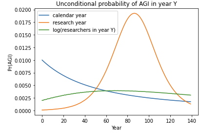
In fact though I don’t favor these researcher-year definitions, for reasons I explain in this appendix.

10.12.4.1.4 Summary of initial behavior of P(n)

We can make P(n) fall off as fast as we like. We can make it fall slow enough that allowing it to fall off slower still wouldn’t affect the bottom line. We can’t make P(n) increase, but we can use the conjunctive model or alternative trial definitions to model potential reasons that P(n) might increase. So overall, it seems that the models discussed in this report are sufficient for the initial behavior of P(n).

10.12.4.2 The framework is sufficiently flexible about how P(n) changes in the tails

With 1 virtual success, P(n) falls off with 1 / (γ + n)². So in the tails, P(n) falls of with 1/n². But there are other mathematical possibilities: P(n) could fall off with 1/nⁱ for any i > 1,186 and there are other functional forms that P(n) could have in the tail.

A semi-informative distribution can express any of the possibilities where P(n) falls off with 1/nⁱ. It turns out that if the number of virtual successes = v, then in the tail P(n) falls off with 1/n^1+v. This result follows from the fact that this framework approximates a Pareto distribution in its tail and the formula for the probability density of a Pareto distribution.

If you have strong intuitions about exactly how fast P(n) should fall off, you could use this to choose the number of virtual successes. I have not explicitly used claims about the tails to constrain the inputs in this document, but I discuss the tail behavior in this appendix.

If you take a weighted sum over different update rules, then in the long run P(n) falls off with the update rule with fewest virtual successes.187 So you can assign some weight to update rule U, and the rest of your weight to update rules with more virtual successes than U, and the behavior in the tails will correspond to the number of virtual successes in U.

10.12.4.3 Given 1-3, the framework is sufficiently general

The main contributors to the shape of P(n) are i) how high it is initially, ii) how it changes initially, and iii) how fast it decreases in the tails. A different framework wouldn’t change any of these things significantly, so wouldn’t significantly change the height of P(n) over the next few decades.

I find this argument somewhat convincing. To object, you’d have to claim that an alternative distribution with a different shape would actually move a substantial amount of probability from one part of the curve to another part.

My response is that the only two possibilities I can think of where this happens are i) probability moving into the tails and ii) probability moving away from the early trials. In answer to (i), our framework allows for an arbitrarily large amount of probability to lie in after the Nth trial for any N: just choose a small enough first-trial probability and number of virtual successes (see diagrams here). In answer to (ii), the conjunctive framework significantly dampens the probability of early trials. So I think other frameworks would make <2X difference to the bottom line.

10.12.5 Potential limitations of the semi-informative framework

I summarize some limitations of the framework, along with my responses.

• The probability of the early trials is unrealistically high – AGI would never have been developed in the first three years of effort.

Move over to the conjunctive model, which dampens early probabilities but gives similar results for later trials. Or (more roughly) choose a later regime start-time so that there might have been enough time to develop AGI between 1956 and the regime start-time.

• The framework isn’t appropriate if we have an end-point by which we’re confident AGI will have been developed.

This is true. In such cases, I recommend using a uniform or normal distribution instead, or searching for another distribution entirely.

• There might be some other probability distribution over trials that is more reasonable and so gives more reasonable results.

I think it’s unlikely that another distribution would output probabilities that differ more than 2X, for reasons I give here and here. However, my argument here is not water-tight. In case anyone is interested to pursue this, I found some distributions that I don’t think can be approximated by my framework and seemed upon a very quick inspection like they might give reasonable distribution over trials:

• Generalized Pareto distribution
• Gamma distribution (or the generalized version)
• Inverse Gaussian distribution
• Lévy distribution
• Log-normal distribution
• Lomax distribution
• Fréchet distribution
• Yule-Simon distribution
• Logarithm distribution
• Nakagami distribution
• Beta prime distribution

Even more than exploring the above distributions, I’d be excited to see people developing more nuanced versions of the ‘conjunctive model’ in which trials must be completed sequentially, or in which AGI has disjunctive requirements (rather than just conjunctive).

• In this framework the number of virtual successes controls how quickly P(n) falls off in the tail. But it has the opposite effect on how quickly P(n) falls off initially. Fewer virtual successes makes P(n) fall off faster initially but more slowly in the tail. What if I want P(n) to fall off slowly both at first and in the tail.

If you specify exactly how quickly P(n) falls off in the tail and how quickly it falls off initially, this determines its starting height. In other words, you’re free to specify at most two of the following three things independently: i) P(1), ii) How quickly P(n) falls off initially, iii) How quickly P(n) falls off in the tail. This is because P(n) sums to 1 over all n. To me, it feels most natural to specify (i) and (ii).

10.12.6 Summary

I’m not excited about improving the bottom line by considering models outside of this framework and the conjunctive model. However, it’s definitely possible I’ve missed something! I spent the vast majority of my time on this project working within the framework, only occasionally thinking about limitations and investigating them a bit more near the end.

10.13 Should we use # virtual successes or # virtual observations as an input to the semi-informative priors framework?

10.13.1 Background

As it stands, the report takes the number of virtual successes to be an input, alongside the first-trial probability. The inputs have the following meanings:

• First-trial probability: How likely you think the first trial is to succeed.
• Virtual successes: How resistant you are to updating away from the first-trial probability when subsequent evidence (of successes or failures) come in.

But another possibility would be to replace ‘virtual successes’ with the total number of virtual observations (both successes and failures).

Virtual observations = virtual successes + virtual failures = virtual successes / first-trial probability.

The resistance to updating increases with both the virtual observations and the virtual successes, so it seems that either could represent the resistance to updating in theory.

10.13.2 Why I prefer to use virtual successes: the update rule for E(p)

E(p) gives your probability that the next trial will succeed. I like to think about the inputs in terms of how E(p) changes over time as we observe more failed trials.

I think that using virtual successes as an input allows us to think about the behavior of E(p) more intuitively than using virtual observations. I’ll explain this by considering the formula for how E(p) changes over time.

Let’s look at the formula for E(p) changes over time, first with virtual successes as an input and then with virtual observations as an input.

Let’s use the following symbols:

• First-trial probability = 1/N
• Virtual successes = s
• Virtual observations = o
  • o = s × N
• Number of observed failed trials = n

10.13.2.1 E(p) formula, virtual successes as an input

\( E(p)=1/(N+n/s) \)

The inverse of E(p) represents (my estimate of) the difficulty of creating AGI. It is simply N + n/s. I can easily separate out the effect of the first-trial probability (N) and the effect of the update from observed failure (n/s). If I vary the first-trial probability, holding virtual successes fixed, I don’t change the size of the update from observed failures (n/s).

10.13.2.2 E(p) formula, virtual observations as an input

\( E(p)=1/(N+Nn/o) \)

This time, I find the inverse of E(p) harder to think about: N + Nn/o. I can’t easily separate out the effect of the first-trial probability (N) and the effect of the update from observed failure (Nn/o). If I vary the first-trial probability, holding virtual observations fixed, I change the size of the update from observed failures Nn/o. So this parameterization seems to make the first-trial probability do double duty as both influencing the initial value of E(p) and the size of the update from failure.

10.13.2.3 A worked example

I want to be able to vary the first-trial probability, holding the other input fixed, without the resistance to updating changing. If I use virtual observations as an input, then (intuitively) the resistance to updating changes significantly when I change the first-trial probability.

10.13.2.3.1 Virtual observations as an input

Suppose we have 20 virtual observations, o = 20. If first-trial probability = 1/2, then N = 2 and

\( E(p)=1/(N+Nn/o)=1/(2+n/10) \)

Initially, E(p) = 1/2. After observing 10 failed trials, E(p) = ⅓. After 20 failures, E(p) = ¼. Intuitively, I find this to be highly resistant to updating away from the first-trial probability.

Now, let’s change the first-trial probability, holding the other input fixed. We still have o = 20, but this time the first-trial probability = 1/500.

\( E(p)=1/(500+25n) \)

Initially, E(p) = 1/500. After observing 10 failed trials, E(p) = 1/750. After 20 failures, E(p) = 1/100. Intuitively, I find this to be extremely non-resistant to updating away from the first-trial probability. The 20 observed failures were not at all surprising, and yet you updated very significantly.

So we see that the intuitive ‘resistance to updating’ changes significantly when we hold the virtual observations fixed and change the first-trial probability. This is very undesirable, as I don’t want the first-trial probability to influence the resistance to updating.

10.13.2.3.2 Virtual successes as an input

I don’t find this problem arises when we take virtual successes to be an input. Suppose we have 10 virtual successes, s = 10. Then when first-trial probability = 1/2, we have:

\( E(p)=1/(N+n/s)=1/(2+n/10) \)

Initially, E(p) = 1/2. After observing 10 failed trials, E(p) = ⅓. After 20 failures, E(p) = ¼. Intuitively, I find this to be highly resistant to updating away from the first-trial probability. This is just the same as above.

Now, let’s change the first-trial probability, holding the other input fixed. We still have s = 10, but this time the first-trial probability = 1/500

\( E(p)=1/(500+n/10) \)

Initially, E(p) = 1/500. After observing 10 failed trials, E(p) = 1/501. After 20 failures, E(p) = 1/503. Intuitively, I find this to be highly resistant to updating away from the first-trial probability. In other words, I find the degree of resistance to updating to be intuitively similar when the first-trial probability is 1/2 as when it is 1/500. So in this case, the intuitive ‘resistance to updating’ does not change significantly when we hold the virtual observations fixed and change the first-trial probability. This is desirable.

10.14 Inputs for low-end, central, and high-end final calculations

10.14.1 Low

TRIAL DEFINITION	OTHER PARAMETERS	INITIAL WEIGHT
Calendar-year	Virtual successes: 0.5 Regime start: 1956 First trial probability: 1/1000	50%
Research-year	Virtual successes: 0.5 Regime start: 1956 ftpcal: 1/1000 gexp : 4.3% gact : 7%	30%
AGI is impossible		20%

10.14.2 Central

TRIAL DEFINITION	OTHER PARAMETERS	INITIAL WEIGHT
Calendar-year	Virtual successes: 1 Regime start: 1956 First trial probability: 1/300	30%
Research-year	Virtual successes: 1 Regime start: 1956 ftpcal: 1/300 gexp : 4.3% gact : 11%	30%
Compute	Virtual successes: 1 2036 spend: $1bn Method for ftp: ‘relative importance of research and compute’ X: 5 gexp : 4.3% Regime start: 1956 ($1 spend on compute at 1956 FLOP/$) ftpcal: 1/300	5%
Compute	Virtual successes: 1 2036 spend: $1bn Method for ftp: lifetime bio-anchor Regime start: 1956 ($1 spend on compute at 1956 FLOP/$)	10%
Compute	Virtual successes: 1 2036 spend: $1bn Method for ftp: evolution bio-anchor Regime start-time: the regime starts when we first use “brain debugging computation” (1021 FLOPS) to develop an AI system.	15%
AGI is impossible		10%

10.14.3 High

TRIAL DEFINITION	OTHER PARAMETERS	INITIAL WEIGHT
Calendar-year	Virtual successes: 1 Regime start: 2000 First trial probability: 1/100	10%
Researcher-year	Virtual successes: 1 Regime start: 2000 ftpcal: 1/100 gexp : 4.3% gact : 11%	40%
Compute	Virtual successes: 1 2036 spend of $100 billion (aggressive) X: 5 gexp: 4.3% gact: 16% ftpcal: 1/100 Regime start: 1956 ($1 spend on compute at 1956 FLOP/$)	10%
Compute	Virtual successes: 1 2036 spend: $100 billion (aggressive) Bio-anchor: lifetime Regime start: 1956 ($1 spend on compute at 1956 FLOP/$)	10%
Compute	Virtual successes: 1 2036 spend: $100 billion (aggressive) Bio-anchor: evolution Regime start-time: the regime starts when we first use “brain debugging computation” (1021 FLOPS) to develop an AI system.	20%
AGI is impossible		10%

10.15 Links to reviewer responses

The report was reviewed by three academics. Here are links to their reviews, to which I have appended my responses:

• Alan Hajek and Jeremy Strasser
• Robin Hanson
• Joe Halpern

11 Supplementary Materials

MATERIAL	SOURCE
How often do tech events as impactful as AGI occur?	Source
Don’t rule out AGI in the first 100 years of trying	Source
Don’t expect too many very high impact technologies to be developed	Source
Anchor off maths proofs	Source

12 Sources

DOCUMENT	SOURCE
Aghion (2017)	Source
AI Impacts, “AI conference attendance”	Source
AI Impacts, “Wikipedia history of GFLOPS costs”	Source
AI Impacts, “Resolutions of mathematical conjectures over time”	Source
Baum (2017)	Source
Bloom (2017)	Source
Bloom (2020)	Source
Bostrom (2014)	Source
Carlsmith (2020a)	Source
Carlsmith (2020b)	Source
Cotra (2020)	Source
Cotton-Barratt (2014)	Source
Deng et al. (2009)	Source
Drexler (2019)	Source
Effective Altruism Concepts, “Credences”	Source
Fallenstein and Mennen (2013)	Source
Grace (2017)	Source
Gruetzemacher (2020)	Source
Gwern (2019)	Source
Hanson (2001)	Source
Human Center for Artificial Intelligence, “Artificial Intelligence Index Report 2018”	Source
Human Center for Artificial Intelligence, “Artificial Intelligence Index Report 2019”	Source
JF Gagne, “Global AI Talent Report 2019”	Source
Jones (1995)	Source
Jones (1998)	Source
Jones (1999)	Source
Karnofsky (2016)	Source
Kremer (1993)	Source
Lee (1988)	Source
LessWrong, “Inside/Outside View”	Source
Li (2020)	Source
McCarthy et al. (1955)	Source
Muehlhauser (2013)	Source
OECD AI, “Live data from partners”	Source
Open Philanthropy, “Ajeya Cotra”	Source
Open Philanthropy, “Holden Karnofsky”	Source
Open Philanthropy, “Joseph Carlsmith”	Source
OpenAI (2018)	Source
OpenAI (2020)	Source
OpenAI et al. (2020)	Source
OpenAI, Landing Page	Source
Raman (2000)	Source
Random, “7. The Beta-Bernoulli Process”	Source
Roodman (2020)	Source
Russell (2019)	Source
Shlegeris (2020)	Source
Sinick (2013)	Source
Stanford Encyclopedia of Philosophy, “Dutch Book”	Source
Stanford Encyclopedia of Philosophy, “Hans Reichenbach”	Source
Sutton (2019)	Source
Tardi (2020)	Source
Vincent (2017)	Source
Vollrath (2019)	Source
Weitzman (1997)	Source
Wikipedia, “Bayes’ Theorem”	Source
Wikipedia, “Bayesian inference”	Source
Wikipedia, “Bayesian probability”	Source
Wikipedia, “Bernoulli trial”	Source
Wikipedia, “Beta distribution”	Source
Wikipedia, “Beta negative binomial distribution”	Source
Wikipedia, “Beta prime distribution”	Source
Wikipedia, “Beta-binomial distribution”	Source
Wikipedia, “Cobb-Douglas production function”	Source
Wikipedia, “Conjugate prior distribution”	Source
Wikipedia, “DeepMind”	Source
Wikipedia, “Elasticity of substitution”	Source
Wikipedia, “ENIAC”	Source
Wikipedia, “Exponential distribution”	Source
Wikipedia, “Floating-point arithmetic”	Source
Wikipedia, “Fréchet distribution”	Source
Wikipedia, “Gamma distribution”	Source
Wikipedia, “Generalized gamma distribution”	Source
Wikipedia, “Generalized Pareto distribution”	Source
Wikipedia, “Geometric distribution”	Source
Wikipedia, “Gross World Product”	Source
Wikipedia, “History of artificial intelligence”	Source
Wikipedia, “Hyperprior”	Source
Wikipedia, “Inverse Gaussian distribution”	Source
Wikipedia, “Jeffreys prior”	Source
Wikipedia, “Lévy distribution”	Source
Wikipedia, “Log-normal distribution”	Source
Wikipedia, “Logarithmic distribution”	Source
Wikipedia, “Lomax distribution”	Source
Wikipedia, “Moore’s law”	Source
Wikipedia, “Nakagami distribution”	Source
Wikipedia, “Negative binomial distribution”	Source
Wikipedia, “Normal distribution”	Source
Wikipedia, “Pareto distribution”	Source
Wikipedia, “Pierre-Simon Laplace”	Source
Wikipedia, “Prior probability”	Source
Wikipedia, “Reciprocal distribution”	Source
Wikipedia, “Reference class forecasting”	Source
Wikipedia, “Rule of succession”	Source
Wikipedia, “Sunrise problem”	Source
Wikipedia, “Uniform distribution (continuous)”	Source
Wikipedia, “Yule-Simon distribution”	Source
Wikipedia, “Superintelligence: Paths, Dangers, Strategies”	Source
Zabell (2009)	Source