• Partner With Us
  • Focus Areas
    • Cause Selection
    • Global Health & Wellbeing
      • Abundance & Growth
      • Effective Giving & Careers
      • Farm Animal Welfare
      • Global Aid Policy
      • Global Health & Development
      • Global Health R&D
      • Global Public Health Policy
      • Scientific Research
    • Global Catastrophic Risks
      • Biosecurity & Pandemic Preparedness
      • Forecasting
      • Global Catastrophic Risks Capacity Building
      • Potential Risks from Advanced AI
    • Other Areas
      • History of Philanthropy
  • Grants
  • Research & Updates
    • Blog Posts
    • In the News
    • Research Reports
    • Notable Lessons
  • About Us
    • Grantmaking Process
    • How to Apply for Funding
    • Careers
    • Team
    • Operating Values
    • Stay Updated
    • Contact Us
  • Partner With Us
  • Focus Areas
    • Cause Selection
    • Global Health & Wellbeing
      • Abundance & Growth
      • Effective Giving & Careers
      • Farm Animal Welfare
      • Global Aid Policy
      • Global Health & Development
      • Global Health R&D
      • Global Public Health Policy
      • Scientific Research
    • Global Catastrophic Risks
      • Biosecurity & Pandemic Preparedness
      • Forecasting
      • Global Catastrophic Risks Capacity Building
      • Potential Risks from Advanced AI
    • Other Areas
      • History of Philanthropy
  • Grants
  • Research & Updates
    • Blog Posts
    • In the News
    • Research Reports
    • Notable Lessons
  • About Us
    • Grantmaking Process
    • How to Apply for Funding
    • Careers
    • Team
    • Operating Values
    • Stay Updated
    • Contact Us

Extreme Risks from Climate Change

  • Content Type: Research Reports

Table of contents

In a nutshell

1. The problem: Risk of worse-than-expected impacts

1.1 Examples of low-probability, high-impact risks

2. What are possible interventions?

3. Who else is working on it?

4. Questions for further investigation

5. Our process

6. Sources

Published: November 23, 2013

In a nutshell

In our main discussion of the impacts of unmitigated climate change, we focused on summarizing the most likely outcomes according to the Intergovernmental Panel on Climate Change.1 However, the dynamics of climate change are such that low-probability, extremely harmful impacts can dominate estimates of the overall harms. Only accounting for the most likely impacts of climate change, accordingly, may lead to a significant underestimate of the total expected impacts.2 This page reviews our understanding of extreme humanitarian risks of climate change that are considered possible but unlikely, and considers interventions that may mitigate those risks. This page is one part of our broader shallow investigation of how climate change may compare to other philanthropic opportunities.


1. The problem: Risk of worse-than-expected impacts

The Intergovernmental Panel on Climate Change Fourth Assessment Report considers a global average temperature increase of 2.4-6.4ºC by 2100 to be “likely” under a high emissions scenario.3 Based on the IPCC’s technical definition of “likely,” we take this assessment to mean that the expert consensus cannot rule out a very meaningful–around 10%–chance of a global average temperature increase of more than 6.4ºC by 2100, though we understand the upper confidence limit on temperature increase to be highly uncertain.4 Such a large temperature increase may be disastrous for large populations of people.5 The risk of greater-than-expected temperature change is worth particular attention because the estimated humanitarian impacts of climate changes are highly nonlinear: marginal temperature increases are expected to cause more damage at already-increased temperatures (i.e. going from 3ºC to 4ºC is expected to be significantly worse than going from 1ºC to 2ºC). This implies that the “likely” impacts considered on our main page on the impacts of climate change–and, largely, by scientists and the IPCC–may vastly understate the true expected value of climate change harms. For instance, on the fairly common, though not necessarily well-grounded, assumption that damages from climate change are roughly proportional to the square of temperature change, a 10% risk of a 6.4ºC temperature increase would be approximately as harmful as a 100% risk of a 2ºC temperature increase.6 The humanitarian risk due to worse-than-expected climate change may be even larger than this example suggests, for two reasons:

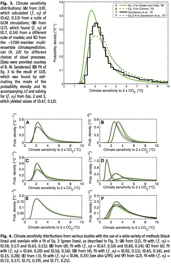
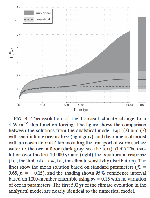
  1. Uncertainty about climate sensitivity is asymmetrically distributed in a way that favors more extreme temperature changes, and potentially very extreme climate changes can’t be ruled out.7 Further observation may be unable to reduce this uncertainty much.8 However, in the event of very high climate sensitivity (i.e. a high degree of climate change for the level of carbon in the atmosphere), our understanding is that the full temperature increase will likely take centuries to occur because the oceans absorb heat at a relatively slow pace.9 Accordingly, the uncertainty in the upper tail of the climate sensitivity distribution primarily impacts expected temperatures in the distant future.
  2. More importantly, the damage caused by a given change in temperature is unlikely to follow precisely the hypothesized quadratic relationship, and may well be far worse than quadratic for high temperature changes.10 Modeling uncertainty and “unknown unknowns” further widen the bands of uncertainty around potential harms.11

Note: this page was drafted prior to the release of the Fifth Assessment Report of the First Working Group of the IPCC in September 2013. The Fifth Assessment Report continues to support the general conclusions reported above, though it reports a slightly narrower confidence interval for temperature change in 2100 under the highest included emissions scenario, primarily because of a change in scenario composition.12 This discussion has been limited and conceptual. Below, we review a few non-systematic examples of how damages from worse-than-expected outcomes could play an important role in an overall assessment of the harms of climate change.

1.1 Examples of low-probability, high-impact risks

Climate change could potentially trigger a number of low-probability environmental events with extremely adverse consequences to humans. One such risk is the melting of the Greenland ice sheet, leading to sea level rise and flooding.13 Our understanding, discussed on our main page on climate impacts, is that sea level rise of more than 2 meters in the 21st century is considered unlikely, and that, with adaptation, such a sea level rise is projected to displace roughly 300,000 people, while without adaptation, it is projected to displace nearly 200 million people.14 However, climate scientist James Hansen has questioned this upper limit and argued that the 21st century could see as much as five meters of sea level rise.15 We do not have a quantitative assessment of the probability of such a radical level of sea level rise, and we believe it to be widely considered unlikely, but we are not in a position to rule it out at this point. Rising temperatures could also impact human health through extreme heat waves, or cause droughts that might lead to water scarcity and decreased agricultural production.16 More extremely, we have seen it argued that a 12ºC increase in mean global temperature—which is substantially outside the range considered plausible this century—would cause at least one day each year in the territories where half of all people live today to be hot enough to exceed human metabolic limits and cause tissue damage from hyperthermia after a few hours of exposure.17 More likely, and on a shorter time-scale, climate change may have severe second-order impacts on human welfare, such as conflict over newly scarce resources or over the use of a controversial mitigation strategy such as geoengineering.18 These examples are only a few of the many possible low-probability, high-impact results of climate change that may play an important role in the overall harms of climate change.19 Since uncertainty compounds at each level from temperature changes to first-order effects to second-order effects, the overall probability that climate change will have catastrophic negative effects on human welfare is very uncertain. This uncertainty makes it hard to dismiss extreme risks on the basis of their low probability.20


2. What are possible interventions?

Reductions in greenhouse gas emissions are expected to disproportionately reduce the risk of extreme temperature increases and extreme impacts (relative to how much they reduce median estimated temperature changes), so mainstream interventions to reduce the negative impacts of climate change in general (discussed on our page on anthropogenic climate change) may be the most effective strategy for addressing extreme risks.21 A funder could also focus on efforts that are more specific to extreme risks, such as:

  • Geoengineering research. Geoengineering using solar radiation management might seem more attractive under more extreme climate change, because extreme effects might be seen to justify the risks of geoengineering.22 Research on geoengineering could conceptually help policymakers make a more informed decision in an extreme situation. (See our page on geoengineering research for more.)
  • Further research on extreme climate change. Additional research could help reduce uncertainty and inform mitigation or adaptation. Empirical research on the rate of ice and permafrost melting and integrated modeling of interrelated and multilevel climate change effects may be particularly promising.23 However, some climate scientists have suggested that reducing uncertainty about individual feedbacks may not appreciably reduce uncertainty about the overall impacts of climate change.24

3. Who else is working on it?

See our main page on climate change for groups working to address climate change, and our page on geoengineering research for groups working on geoengineering research. We believe that funding for research on extreme climate change comes mostly from basic science funders like the National Science Foundation, as well as from some private donors.25 However, we do not have an overall estimate of the amount of funding in this area.


4. Questions for further investigation

Our research in this area has been relatively limited, and we have yet to answer many important questions. Amongst other topics, our further research on this cause might address:

  • What concrete funding opportunities exist to limit extreme risks from climate change?
  • What areas of further scientific research are most likely to reduce uncertainty around extreme risks from climate change? To what extent is it possible to reduce such uncertainties?
  • How much are other funders spending on various initiatives to work on extreme risks from climate change?
  • How does the value of work to specifically limit extreme climate risks compare to more common efforts to limit overall climate changes?

5. Our process

We decided to look into extreme risks from climate change because our initial review of climate impacts based on the IPCC’s Fourth Assessment report mostly focused on likely outcomes of climate change, and we saw research suggesting that low-probability, severe impacts can dominate estimates of harms due to climate change.26 We read a number of papers on various aspects of extreme climate risks, particularly focusing on economic models, and spoke to three academics in the field:

  • Elmar Kriegler – Senior Scientist at the Potsdam Institute for Climate Impact Research
  • Kirsten Zickfeld – Assistant Professor, Simon Fraser University, Department of Geography
  • Klaus Keller – Associate Professor of Geosciences, Pennsylvania State University

6. Sources

DOCUMENT SOURCE
Baker and Roe 2009 Source (archive)
Hansen and Sato 2012 Source (archive)
IPCC AR4 Synthesis Report Source (archive)
IPCC AR4 WGI Chapter 10 Source (archive)
IPCC AR5 WGI Chapter 12 Source (archive)
IPCC AR5 WGI Summary for Policymakers Source (archive)
Kelly and Tan 2013 Source (archive)
Kousky et al. 2010 Source (archive)
Mendelsohn 2009 Source (archive)
Nicholls et al. 2011 Source (archive)
Notes from a conversation with Elmar Kriegler, 4/18/2013 Source
Notes from a conversation with Kirsten Zickfeld, 04/17/13 Source
Notes from a conversation with Klaus Keller, 4/18/2013 Source
Roe and Baker 2007 Source (archive)
Roe and Bauman 2012 Source (archive)
Sherwood and Huber 2010 Source (archive)
Stanton, Ackerman, and Kartha 2008 Source (archive)
Weitzman 2009 Source (archive)
Weitzman 2012 Source (archive)
Expand Footnotes Collapse Footnotes

1.We did take into account information about the full distribution of expected impacts when it was available, such as in the case of economic projections of climate impacts (which are meant to capture the possibility of worse than anticipated harms), but it was not normally available in the IPCC reports.

2.Weitzman 2009.

3.Scenario A1Fl, IPCC AR4 Synthesis Report, pg. 45.

4.

“Where uncertainty in specific outcomes is assessed using expert judgment and statistical analysis of a body of evidence (e.g. observations or model results), then the following likelihood ranges are used to express the assessed probability of occurrence: virtually certain > 99%; extremely likely > 95%; very likely > 90%; likely > 66%; more likely than not > 50%; about as likely as not 33% to 66%; unlikely < 33%; very unlikely < 10%; extremely unlikely < 5%; exceptionally unlikely < 1%.” IPCC AR4 Synthesis Report, pg. 27.

If the “likely” range of temperature changes covers between 66% and 90% of the assessed probability of temperature changes, then we would expect between 5% and roughly 17% of the probability distribution to fall on a change of >6.4ºC.

“The AOGCMs cannot sample the full range of possible warming, in particular because they do not include uncertainties in the carbon cycle. In addition to the range derived directly from the AR4 multi-model ensemble, Figure 10.29 depicts additional uncertainty estimates obtained from published probabilistic methods using different types of models and observational constraints: the MAGICC SCM and the BERN2.5CC coupled climate-carbon cycle EMIC tuned to different climate sensitivities and carbon cycle settings, and the C4MIP coupled climate-carbon cycle models. Based on these results, the future increase in global mean temperature is likely to fall within –40 to +60% of the multi-model AOGCM mean warming simulated for each scenario. This range results from an expert judgement of the multiple lines of evidence presented in Figure 10.29, and assumes that the models approximately capture the range of uncertainties in the carbon cycle. The range is well constrained at the lower bound since climate sensitivity is better constrained at the low end (see Box 10.2), and carbon cycle uncertainty only weakly affects the lower bound. The upper bound is less certain as there is more variation across the different models and methods, partly because carbon cycle feedback uncertainties are greater with larger warming. The uncertainty ranges derived from the above percentages for the warming by 2090 to 2099 relative to 1980 to 1999 are 1.1°C to 2.9°C, 1.4°C to 3.8°C, 1.7°C to 4.4°C, 1.4°C to 3.8°C, 2.0°C to 5.4°C and 2.4°C to 6.4°C for the scenarios B1, B2, A1B, A1T, A2 and A1FI, respectively.” IPCC AR4 WGI Chapter 10.

5.“Even without extreme effects, a world with a rise in temperature of approximately 4ºC over the next century would be very different than our current one. As we are adapted to the current climate, the impact could be large, despite the wide range of climates humans already live in. A fast change could be difficult to adapt to, and dealing with it might require lifestyle changes in many parts of the globe (e.g. spending more time indoors, needing infrastructure such as air conditioning, loss of water sources could lead to a need for expensive desalination plants). The impacts on regions without the resources to cope could be severe.” Notes from a conversation with Elmar Kriegler, 4/18/2013.

6.

“Modeling climate economics requires the projection of damages at temperatures outside the historical experience. Many models arbitrarily assume that damages grow as the square of temperature change, calibrated to one or two speculative point estimates of low-temperature damages. Almost all models treat climate damages as losses of current income rather than decreases in capital stock. Alternative assumptions, which are at least as plausible, would lead to much greater estimates of damages, and more urgency about policies to address the problem.” Stanton, Ackerman, and Kartha 2008 pg. 19.

“Economic analyses of impacts also reveal that they follow a dynamic path, increasing roughly by the square of temperature change (Tol 2002b; Mendelsohn and William 2007).” Mendelsohn 2009, pg. 11.

“The most popular single formulation of a damages function in the literature is the quadratic form C(T)=1/[1+(T/α)2], where α is a positive temperature-scaling parameter calibrated to give some “reasonable” values of C(T) for relatively small warmings, say up to T ≈ 2.5◦C. Standard estimates of α in the literature are more or less similar, although I hasten to add that such calibrations were intended by the authors to capture low-temperature damages and were never intended to be extrapolated to very high temperature changes, which is just what I will be doing here. For the sake of having a specific prototype example, I calibrate α in Equation (7) to conform with the damages function in the latest version of the well known DICEmodel of William Nordhaus (2008), where he effectively used α = 20.46. In this case, welfare equivalent consumption is given by the formula C( T ) = 1/[1+(T/20.46)2] where the natural scaling factor for T is the rather large temperature α = 20.46◦C.” Weitzman 2012, pg. 223.

Using the formula given by Weitzman 2012 to characterize Nordhaus’ DICE damage function, a 100% chance of a 2ºC temperature increase would reduce welfare by about 0.95%, while a 10% chance of a 6.4ºC change would reduce welfare by 0.89% (since a 6.4ºC change would reduce welfare by 8.9%).

7.

“Glancing at table 9.3 and box 10.2 of IPCC-AR4, it is apparent that the upper tails of these 22 PDFs [probability density functions] tend to be sufficiently long and fat that one is allowed from a simplistically aggregated PDF of these 22 studies the rough approximation P[S1 > 10ºC] ≈ 1%. The actual empirical reason why these upper tails are long and fat dovetails beautifully with the theory of this paper: inductive knowledge is always useful, of course, but simultaneously it is limited in what it can tell us about extreme events outside the range of experience—in which case one is forced back onto depending more than one might wish upon the prior PDF, which of necessity is largely subjective and relatively diffuse. As a recent Science commentary put it: ‘Once the world has warmed by 4°C, conditions will be so different from anything we can observe today (and still more different from the last ice age) that it is inherently hard to say where the warming will stop.’” Weitzman 2009, pg. 3.

Roe and Baker 2007, pg. 631.

8.

“We have shown that the uncertainty in the climate sensitivity in 2 × CO2 studies is a direct and general result of the fact that the sum of the underlying climate feedbacks is substantially positive. Our derivation of hT (DT) did not depend on nonlinear, chaotic behavior of the climate system and was independent of details in cloud and other feedbacks. Equation 3 appears to explain the range of climate sensitivities reported in previous studies, which are well synthesized by the IPCC (1). Furthermore, reducing the uncertainty in individual climate processes has little effect in reducing the uncertainty in climate sensitivity. We do not therefore expect the range presented in the next IPCC report to be greatly different from that in the 2007 report. On the basis of the values of f and sf compiled from our analysis of a large number of published results, it is evident that the climate system is operating in a regime in which small uncertainties in feedbacks are highly amplified in the resulting climate sensitivity. We are constrained by the inevitable: the more likely a large warming is for a given forcing (i.e., the greater the positive feedbacks), the greater the uncertainty will be in the magnitude of that warming.” Roe and Baker 2007, pg. 632.

However, other authors appear to disagree: “Our results show that the social planner rejects that the climate sensitivity is in the upper tail of the prior distribution very quickly. That is, although we confirm results in the previous literature that learning the actual true value precisely is a relatively slow process, the planner is able to reject values of the climate sensitivity in the upper tail of the prior distribution quickly. In fact, the planner can reject very high values of the climate sensitivity (e.g. 1.5°C or more above the mean estimate) at 99% confidence interval in less than a decade, if the true climate sensitivity is moderate. First, observations near the moderate true value provide evidence against the tails of the distribution. In addition, the density of even a fat tail is not large, so Bayes rule requires relatively few observations to reduce the mass of the fat tail below the critical confidence level. This result is surprising given the common intuition in the literature that reducing uncertainty in the tail of the climate sensitivity prior distribution must be a slow process since climate disasters are rare (see for example, Weitzman 2009, page 12). If the true climate sensitivity turns out to be relatively high, learning progresses more slowly. First, Bayes rule requires more observations to move the mean estimate from the prior of a moderate climate sensitivity to the true high value. Second, Bayes rule requires more observations to resolve the difference between a climate sensitivity that is relatively high and a climate sensitivity which is very high. Nonetheless, because a high climate sensitivity is relatively unlikely according to the prior, the possibility that learning is slower due to a high climate sensitivity receives relatively little weight when computing the expected time until partial learning is complete… In terms of optimal policy, we quantify the effect of uncertainty on near term emissions and abatement policy. With uncertainty but without learning, in the initial period emissions are about 38% lower, and the carbon tax is $22.94 higher, than under certainty. The planner insures by reducing emissions, paying for more abatement to reduce the probability of high damages that occur if the climate sensitivity is high. However, in the current period, emissions with uncertainty and learning are only about 19% lower than under certainty. The optimal carbon tax with uncertainty and learning is only $8.84 per ton higher than under certainty. Therefore, learning reduces emissions abatement for insurance purposes by about 50%. Further, optimal emissions with uncertainty and learning converge quickly to emissions given perfect information, typically in about 16 years. Uncertainties remain after 16 years, but the remaining uncertainty is not relevant for the optimal emissions policy. The fat tail drives policy, and learning shrinks the mass of the fat tail quickly.9 ” Kelly and Tan 2013, pgs 3-4.

9.

“I want to state clearly and emphatically here, once and for all, that very high atmospheric temperature changes like T = 12◦C will likely take millennia to attain. The higher the limiting temperature, the longer it takes to achieve atmospheric equilibrium because the oceans will first have to absorb the enormous amounts of heat being generated. Alas, building up such enormous amounts of heat in the ocean is like compressing a very powerful coiled spring. It could set in motion nasty surprises, such as long-term methane clathrate releases from the continental shelves, whose possibly horrific consequences are essentially irreversible and would have to be dealt with later. For the toy model of this paper, overall damages generated by equilibrium T = 12◦C are best conceptualized as associated with being on the trajectory whose asymptotic limiting atmospheric temperature change is T = 12◦C. It is important to bear this interpretation in mind, even though a discrete date will be assigned for the “as if ” transition to higher temperatures in the toy model.” Weitzman 2012 pg 230.

Baker and Roe 2009, pg. 4578.

10.“All damage functions are made up—especially for extreme situations. Therefore, neither I nor anyone else has an objective basis for determining magnitudes of high-temperature damages. I now want to “give the devil his due” by characterizing very roughly two points on a much more reac- tive global damages function, which seems to me far more plausible than the quadratic and which attributes far bigger welfare-equivalent damages to higher temperatures. Of course no one knows how to estimate welfare- equivalent damages for very high temperature changes. I anchor my “give the devil his due” damages function on the two “iconic” (if arbitrary) global- average temperature changes: 6◦C and 12◦C. What these two iconic global warmings might mean for the human condition and for the rest of the planet has already been sketched out. At 6◦C I propose welfare-equivalent consumption of CR(6◦C) = 50% (at that time), while for 12◦C I propose welfare- equivalent consumption of CR (12◦ C) = 1%. I do not consider such estimates to be extreme when interpreted as welfare-equivalent damages to a fictitious agent representing the entire planet, although others may disagree and are free to substitute their own guesstimates.” Weitzman 2012, pg 234.

11.

“Unabated emissions of greenhouse gases could result in catastrophic climate change impacts for some. Potential climate stressors driving these impacts include warming (e.g., via health impacts), drought (e.g., via agriculture impacts), and sea level rise (e.g., via displacement and potential for conflicts). Projections of climate change impacts are deeply uncertain. Characterizing this uncertainty is an active research area.” Notes from a conversation with Klaus Keller, 4/18/2013.

“Much more unsettling for an application of (present discounted) expected utility analysis are the unknowns: deep structural uncertainty in the science coupled with an economic inability to evaluate meaningfully the catastrophic losses from disastrous temperature changes. The climate science seems to be saying that the probability of a disastrous collapse of planetary welfare is nonnegligible, even if this tiny probability is not objectively knowable” Weitzman 2009, p. 1.

12.

IPCC AR5 WGI Summary for Policymakers Table 2 reports a mean temperature change for scenario RCP 8.5 of 3.7ºC in 2081-2100 relative to 1986-2005, with a “likely” range from 2.6ºC to 4.8ºC. The table includes the note on the confidence intervals, “Calculated from projections as 5−95% model ranges. These ranges are then assessed to be likely ranges after accounting for additional uncertainties or different levels of confidence in models. For projections of global mean surface temperature change in 2046−2065 confidence is medium, because the relative importance of internal variability, and uncertainty in non-greenhouse gas forcing and response, are larger than for 2081−2100. The likely ranges for 2046−2065 do not take into account the possible influence of factors that lead to the assessed range for near-term (2016−2035) global mean surface temperature change that is lower than the 5−95% model range, because the influence of these factors on longer term projections has not been quantified due to insufficient scientific understanding.”

“The uncertainty estimate in AR4 for the SRES scenarios was –40% to +60% around the CMIP3 means (shown here in grey for comparison). That range was asymmetric and wider for the higher scenarios because it included the uncertainty in carbon cycle climate feedbacks. The SRES scenarios are based on the assumption of prescribed emissions, which then translates to uncertainties in concentrations that propagate through to uncertainties in the temperature response. The RCP scenarios assume prescribed concentrations. For scenarios that stabilize (RCP2.6) that approach of constant fractional uncertainty underestimates the uncertainty and is no longer applicable, mainly because internal variability has a larger relative contribution to the total uncertainty (Good et al., 2013; Knutti and Sedláček, 2013). For the RCPs, the carbon cycle climate feedback uncertainty is not included because the simulations are driven by concentrations. Furthermore, there is no clear evidence that distribution of CMIP5 global temperature changes deviates from a normal distribution. For most other variables the shape of the distribution is unclear, and standard deviations are simply used as an indication of model spread, not representing a formal uncertainty assessment. Simulations with prescribed CO2 emissions rather than concentrations are only available for RCP8.5 (Figure 12.8b) and from MAGICC. The projected temperature change in 2100 is slightly higher and the uncertainty range is wider as a result of uncertainties in the carbon cycle climate feedbacks. The CMIP5 range is consistent with the uncertainty range given in AR4 for SRES A2 in 2100. Further details about emission vs. concentration driven simulations are given in Section 12.4.8. In summary, the projected changes in global temperature for 2100 in the RCP scenarios are very consistent with those obtained by CMIP3 for SRES in IPCC AR4 (see Section 12.4.9) when taking into account the differences in scenarios. The likely uncertainty ranges provided here are similar for RCP4.5 and RCP6.0 but narrower for RCP8.5 compared to AR4. There was no scenario as low as RCP2.6 in AR4. The uncertainties in global temperature projections have not decreased significantly in CMIP5 (Knutti and Sedláček, 2013), but the assessed ranges cannot be compared between AR4 and AR5. The main reason is that uncertainties in carbon cycle feedbacks are not considered in the concentration driven RCPs. In contrast, the likely range in AR4 included those. The assessed likely ranges are therefore narrower for the high RCPs. The differences in the projected warming are largely attributable to the difference in scenarios (Knutti and Sedláček, 2013), and the change in the future and reference period, rather than to developments in modeling since AR4. A detailed comparison between the SRES and RCP scenarios and the CMIP3 and CMIP5 models is given in Section 12.4.9.” IPCC AR5 WGI Chapter 12 pg 29.

13.“If the global temperature increases by more than 2-3°C, it is more likely than not that will result in all of the ice in Greenland melting. However, this would take several centuries. Over the next 100 years, the rise in seal level coming from Greenland’s ice melting is expected to be no larger than 0.5 meters. Nevertheless, the sea level rise contribution from the Greenland ice sheet could start to be significant by ~2050. The primary impact that ice melting would have is that the earth’s sea levels would rise. This would have a negative impact on communities that live in low-lying areas, including some communities in North Africa, Asia (for example, in Bangladesh), and the Pacific Islands. In particular, • Coastal assets and infrastructure could be damaged. • People could be displaced from their homes. • The flooding caused by typhoons and hurricanes could increase. • The fresh water on the Pacific Islands could be contaminated by salty water, depriving islander communities of drinkable water.” Notes from a conversation with Kirsten Zickfeld, 04/17/13.

14.Nicholls et al. 2011

15.Hansen and Sato 2012:

“However, the fundamental issue is linearity vs. non-linearity. Hansen (2005, 2007) argues that amplifying feedbacks make ice sheet disintegration necessarily highly nonlinear and that IPCC’s BAU forcing is so huge that it is difficult to see how ice shelves would survive. As warming increases, the number of ice streams contributing to mass loss will increase, contributing to a nonlinear response that should be approximated better by an exponential than by a linear fit. Hansen (2007) suggested that a 10-year doubling time was plausible and pointed out that such a doubling time, from a 1-mm/year ice sheet contribution to sea level in the decade 2005–2015, would lead to a cumulative 5-m sea level rise by 2095.” pg 40

“Debating what sea level will be on a specific date such as 2100, however, misses an important point concerning response times. The carbon cycle response time, i.e., the time required for CO2 from fossil fuel burning to be removed from the surface carbon reservoirs, is many millennia (Berner 2004; Archer 2005). The ice sheet response time is clearly shorter than this carbon cycle response time, in view of the absence of a discernable lag between paleoclimate forcings and the maximum rate of ice sheet disintegration (Hansen et al. 2007a) and in view of the fact that ice sheet disintegration proceeds at rates up to several meters of sea level rise per century (Fairbanks 1989) even in response to weak paleoclimate forcings. Thus, burning all or most fossil fuels guarantees tens of meters of sea level rise, as we have shown that the eventual sea level response is about 20 m of sea level for each degree Celsius of global warming. We suggest that ice sheet disintegration will be a nonlinear process, spurred by an increasing forcing and by amplifying feedbacks, which is better characterized by a doubling time for the rate of mass disintegration, rather than a linear rate of mass change. If the doubling time is as short as a decade, multimeter sea level rise could occur this century. Observations of mass loss from Greenland and Antarctica are too brief for significant conclusions, but they are not inconsistent with a doubling time of a decade or less. The picture will become clearer as the measurement record lengthens. There are physical constraints and negative feedbacks that may limit nonlinear ice sheet mass loss. An ice sheet sitting primarily on land above sea level, such as most of Greenland, may be limited by the speed at which it can deliver ice to the ocean via outlet glaciers. But much of the West Antarctic ice sheet, resting on bedrock below sea level, is not so constrained. We recognize the negative feedback that comes into play as iceberg discharge reaches a rate that cools the regional ocean surface. But that negative feedback would be cold comfort. High-latitude cooling and low-latitude warming would drive more powerful mid-latitude cyclonic storms, including more frequent cases of hurricane force winds. Such storms, in combination with rising sea level, would be disastrous for many of the world’s great cities, and they would be devastating for the world’s economic well-being and cultural heritage.” pg 44.

16.

“Unabated emissions of greenhouse gases could result in catastrophic climate change impacts for some. Potential climate stressors driving these impacts include warming (e.g., via health impacts), drought (e.g., via agriculture impacts), and sea level rise (e.g., via displacement and potential for conflicts).” Notes from a conversation with Klaus Keller, 4/18/2013.

”Some possible effects of extreme climate change events are changes in water availability (for instance, as glaciers used as a water source disappear), a spike in food prices, and migration.”Notes from a conversation with Elmar Kriegler, 4/18/2013.

17.

“In principle humans can devise protections against the unprecedented heat such as much wider adoption of air conditioning, so one cannot be certain that TW (Max) = 35 °C would be uninhabitable. But the power requirements of air conditioning would soar; it would surely remain unaffordable for billions in the third world and for protection of most livestock; it would not help the biosphere or protect outside workers; it would regularly imprison people in their homes; and power failures would become life- threatening. Thus it seems improbable that such protections would be satisfying, affordable, and effective for most of humanity. We conclude that a global-mean warming of roughly 7°C would create small zones where metabolic heat dissipation would for the first time become impossible, calling into question their suitability for human habitation. A warming of 11–12 °C would expand these zones to encompass most of today’s human population. This likely overestimates what could practically be tolerated: Our limit applies to a person out of the sun, in gale-force winds, doused with water, wearing no clothing, and not working. A global-mean warming of only 3–4 °C would in some locations halve the margin of safety (difference between TW max and 35 °C) that now leaves room for additional burdens or limitations to cooling. Considering the impacts of heat stress that occur already, this would certainly be unpleasant and costly if not debilitating. More detailed heat stress studies incorporating physiological response characteristics and adaptations would be necessary to investigate this. If warmings of 10°C were really to occur in next three centuries, the area of land likely rendered uninhabitable by heat stress would dwarf that affected by rising sea level. Heat stress thus deserves more attention as a climate-change impact. The onset of TW max > 35 °C represents a well-defined reference point where devastating impacts on society seem assured even with adaptation efforts. This reference point contrasts with assumptions now used in integrated assessment models. Warmings of 10 °C and above already occur in these models for some realizations of the future (33). The damages caused by 10 °C of warming are typically reckoned at 10–30% of world GDP (33, 34), roughly equivalent to a recession to economic conditions of roughly two decades earlier in time. While undesirable, this is hardly on par with a likely near-halving of habitable land, indicating that current assessments are underestimating the seriousness of climate change. ” Sherwood and Huber 2010, pgs 3-4.

“With 100 W of heat generation (a typical resting value), body mass of 75 kg, and specific heat of 3.5 J g−1 K−1, body temperature would increase by about one degree every 45 minutes. It would thus increase from a normal value of 37 °C to 42 °C—a value that begins to cause permanent tissue damage—in roughly four hours, leading to the tolerance times given in the main text. Given standard values for human resting metabolic rate, mass, specific heat, and surface area, wet bulb temperatures of 37 °C would lead to irreversible heat trauma, associated with sustained core temperatures of 42 °C (, 5, 6, 7) within four to six hours of exposure. The presence of solar or infrared heating could shorten this time even if direct sunlight is avoided, especially if there are nearby solar-heated surfaces radiating at temperatures above ambient or scattered sunlight cannot be avoided.” Sherwood and Huber 2010 Supporting Information.

18.

“Some possible effects of extreme climate change events are changes in water availability (for instance, as glaciers used as a water source disappear), a spike in food prices, and migration. All of this could lead to knock-on effects such as failed states and human conflict – although Dr. Kriegler did mention a recent study that claimed that water conflict, at least, rarely has led to war as diplomatic solutions are normally found. Attempts to mitigate climate change damage through geoengineering have the potential to lead to conflict, as geoengineering could be implemented unilaterally rather than through cooperative action.” Notes from a conversation with Elmar Kriegler, 4/18/2013.

“Some extreme events can have secondary consequences that generate substantial additional damage (Muir-Wood and Grossi 2008). Secondary consequences, in turn, can trigger tertiary consequences that further amplify the adverse consequences, and so on. The compounding or amplifying effects of individual adverse impacts would be the result of exceeding the resilience of a number of local socioeconomic systems concurrently. More frail components of socioeconomic systems, such as marginal subsistence agriculture, represent potential places of vulnerability. One example of this type of mega-catastrophe could arise if increased drought from climate change caused a series of local food shortages to occur in close proximity, leading to political instability, a breakdown of civil order, large-scale migration for survival, and regional conflicts that accompany such events. The economic and national security consequences that spill over to other countries could be catastrophic (CNA Corporation 2007). Cascading-event catastrophes could occur much more rapidly than the slower-onset global impacts discussed in the previous subsection.” Kousky et al. 2010, pgs 6-7.

19.Kousky et al. 2010 describes some other potential consequences: “A second category of mega-catastrophe risk involves weakening and other disruptions of ocean currents. This could potentially alter extreme events, enhance sea level rise, severely disrupt ocean ecosystems, and change precipitation patterns, with serious impacts on agriculture as well as other sectors (Schiermeier 2006; Vellinga and Wood 2008). These impacts also are seen anticipated to increase slowly, over many hundreds of years (Schneider et al. 2007). Very large-scale ecosystem disruptions could occur sooner. There is the prospect of continued and expanded changes in vegetation, particularly irreversible conversion of forest to grassland, as well as increased desertification and acidification of the ocean (e.g., Scholze et al. 2006; Smith et al. 2009). Changes in ecosystems resulting from changes in temperature and rainfall incidence and increased climate variability have the potential to cause significant loss of biodiversity as well as impacts on food and forest products production. The IPCC estimates that with global mean temperatures increasing between 2ºC and 3ºC, 20 to 30 percent of species could be at risk of extinction by 2100 (Fischlin et al. 2007). For higher levels of warming, extinction rates could be 20 to 50 percent (Thomas et al. 2004). All of these effects would be exacerbated by a large and rapid warming that also set in motion other factors (such as more rapid melting of heat-reflecting snow cover, or release of liquefied methane from tundra and elsewhere) that cause a further acceleration in climate change.” Pg 6.

20.“When fed into an economic analysis, the great open-ended uncertainty about eventual mean planetary temperature change cascades into yet much greater, yet much more open-ended uncertainty about eventual changes in welfare. There exists here a very long chain of tenuous inferences fraught with huge uncertainties in every link beginning with unknown base-case GHG emissions; then compounded by huge uncertainties about how available policies and policy levers transfer into actual GHG emissions; compounded by huge uncertainties about how GHG-flow emissions accumulate via the carbon cycle into GHG-stock concentrations; compounded by huge uncertainties about how and when GHG-stock concentrations translate into global mean temperature changes; compounded by huge uncertainties about how global mean temperature changes decompose into regional temperature and climate changes; compounded by huge uncertainties about how adaptations to, and mitigations of, climate-change damages are translated into utility changes—especially at a regional level; compounded by huge uncertainties about how future regional utility changes are aggregated—and then how they are discounted—to convert everything into expected-present-value global welfare changes. The result of this immense cascading of huge uncertainties is a reduced form of truly stupendous uncertainty about the aggregate expected-present-discounted utility impacts of catastrophic climate change, which mathematically is represented by a very spread out, very fat-tailed PDF of what might be called ‘welfare sensitivity.’” Weitzman 2009, pgs. 5-6.

21.

Volume of projected emissions affects the top of the confidence interval of expected temperature increase much more so than the bottom: “Figures 14a,b show the 5% and 95% bounds on the PDF of the maximum temperature reached for different parabolic concentration scenarios, examples of which are shown in Fig. 13. The asymmetry of the PDFs is reflected in Fig. 14, in that the upper 95% bound is more sensitive to variations in the maximum concentration than is the lower bound. Figures 14c,d show the effect of halving uncertainty in all model parameters on the 5% and 95% bounds of the climate projections. The range of climate projections for any given concentration scenarios narrows in response to the reduced uncertainty. However the 95% bound on the maximum temperature reached (i.e., Figs. 14a,c) is most sensitive to small changes in the maximum concentration reached.” Baker and Roe 2009, pg. 4585.

Furthermore, as discussed above, expected damages are superlinear in temperature increase.

22.“How to respond to climate change tail-area events such as climate sensitivity? One potential response, analyzed by some, is geoengineering. For example, increasing the aerosol concentration in the stratosphere would increase the Earths albedo and cool, on average, the Earth’s surface. However, this geoengineering approach can have potentially severe negative side effects, such as abrupt warming in case the geoengineering is stopped or changing precipitation patterns. One additional risk associated with geoengineering strategies is a potential for conflict. This is because geoengineering might “succeed” for some, while causing negative effects for others. Who would decide about an appropriate level of geoengineering? Would the decision be arrived at in a civil way?” Notes from a conversation with Klaus Keller, 4/18/2013.

23.

“Some research that would help assess climate change tail risk is • Further empirical measurements of the rates of ice melting at the Earth’s poles and the rate at which methane is escaping from permafrost. • Climate models that take into account ice dynamics, and that model permafrost methane feedback. Research on climate change tail risk is underfunded. There is no dedicated funding for exploring these risks in Canada. There is more funding available in Europe, under the European Union Framework Program” Notes from a conversation with Kirsten Zickfeld, 04/17/13.

“There is a large and growing body of research focusing on specific climate change effects. This is important, as it provides a foundation for our understanding of the Earth system. However, it is also important to understanding how these effects interact. These interactions are typically less well studied. Example of such interaction effects include the interplay between (i) sea-level rise and adaptation (discussed above) and (ii) the ability to adapt to climate change and the motivation to reduce greenhouse gas emissions and/or deploy geoengineering.” Notes from a conversation with Klaus Keller, 4/18/2013.

“Furthermore, knowledge of global governance and regional politics is crucial to analyzing the knock-on effects of climate change and the potential for conflict. Dr. Kriegler referenced a CIA-funded study to identify the indicators of conflict, and found one indicator to be the local political system” Notes from a conversation with Elmar Kriegler, 4/18/2013.

24.“We have shown that the uncertainty in the climate sensitivity in 2 × CO2 studies is a direct and general result of the fact that the sum of the underlying climate feedbacks is substantially positive. Our derivation of hT (DT) did not depend on nonlinear, chaotic behavior of the climate system and was independent of details in cloud and other feedbacks. Equation 3 appears to explain the range of climate sensitivities reported in previous studies, which are well synthesized by the IPCC (1). Furthermore, reducing the uncertainty in individual climate processes has little effect in reducing the uncertainty in climate sensitivity. We do not therefore expect the range presented in the next IPCC report to be greatly different from that in the 2007 report. On the basis of the values of f and sf compiled from our analysis of a large number of published results, it is evident that the climate system is operating in a regime in which small uncertainties in feedbacks are highly amplified in the resulting climate sensitivity. We are constrained by the inevitable: the more likely a large warming is for a given forcing (i.e., the greater the positive feedbacks), the greater the uncertainty will be in the magnitude of that warming.” Roe and Baker 2007, pg. 632.

25.

“Funding for integrated research is coming in part from federal agencies such NSF (which funds SCRiM). Wealthy individuals are also known to support this kind of research.” Notes from a conversation with Klaus Keller, 4/18/2013.

“Research is currently regionally funded (the National Science Foundation (NSF) in US, the European Union in Europe, etc.) and the groups from different continents often don’t have the resources to collaborate.” Notes from a conversation with Elmar Kriegler, 4/18/2013.

26.Weitzman 2009.

Subscribe to new blog alerts
Open Philanthropy
Open Philanthropy
  • We’re Hiring!
  • Press Kit
  • Governance
  • Privacy Policy
  • Stay Updated
Mailing Address
Open Philanthropy
182 Howard Street #225
San Francisco, CA 94105
Email
info@openphilanthropy.org
Media Inquiries
media@openphilanthropy.org
Anonymous Feedback
Feedback Form

© Open Philanthropy 2025 Except where otherwise noted, this work is licensed under a Creative Commons Attribution-Noncommercial 4.0 International License.

We use cookies on our website to give you the most relevant experience by remembering your preferences and repeat visits. By clicking “Accept All”, you consent to the use of ALL the cookies. However, you may visit "Cookie Settings" to provide a controlled consent.
Cookie SettingsAccept All
Manage consent

Privacy Overview

This website uses cookies to improve your experience while you navigate through the website. Out of these, the cookies that are categorized as necessary are stored on your browser as they are essential for the working of basic functionalities of the website. We also use third-party cookies that help us analyze and understand how you use this website. These cookies will be stored in your browser only with your consent. You also have the option to opt-out of these cookies. But opting out of some of these cookies may affect your browsing experience.
Necessary
Always Enabled
Necessary cookies are absolutely essential for the website to function properly. These cookies ensure basic functionalities and security features of the website, anonymously.
CookieDurationDescription
cookielawinfo-checkbox-analytics11 monthsThis cookie is set by GDPR Cookie Consent plugin. The cookie is used to store the user consent for the cookies in the category "Analytics".
cookielawinfo-checkbox-functional11 monthsThe cookie is set by GDPR cookie consent to record the user consent for the cookies in the category "Functional".
cookielawinfo-checkbox-necessary11 monthsThis cookie is set by GDPR Cookie Consent plugin. The cookies is used to store the user consent for the cookies in the category "Necessary".
cookielawinfo-checkbox-others11 monthsThis cookie is set by GDPR Cookie Consent plugin. The cookie is used to store the user consent for the cookies in the category "Other.
cookielawinfo-checkbox-performance11 monthsThis cookie is set by GDPR Cookie Consent plugin. The cookie is used to store the user consent for the cookies in the category "Performance".
viewed_cookie_policy11 monthsThe cookie is set by the GDPR Cookie Consent plugin and is used to store whether or not user has consented to the use of cookies. It does not store any personal data.
Functional
Functional cookies help to perform certain functionalities like sharing the content of the website on social media platforms, collect feedbacks, and other third-party features.
Performance
Performance cookies are used to understand and analyze the key performance indexes of the website which helps in delivering a better user experience for the visitors.
Analytics
Analytical cookies are used to understand how visitors interact with the website. These cookies help provide information on metrics the number of visitors, bounce rate, traffic source, etc.
Advertisement
Advertisement cookies are used to provide visitors with relevant ads and marketing campaigns. These cookies track visitors across websites and collect information to provide customized ads.
Others
Other uncategorized cookies are those that are being analyzed and have not been classified into a category as yet.
SAVE & ACCEPT